Estimating DGSE models with long memory dynamics

(1)

Département des Sciences Économiques

de l'Université catholique de Louvain

Estimating DGSE models with long memory

dynamics

G. Moretti and G. Nicoletti

Discussion Paper 2008-37

(2)

Estimating DSGE models with long memory

dynamics

Gianluca Moretti and Giulio Nicoletti

∗

Abstract

Recent literature claims that key variables such as aggregate productiv-ity and inflation display long memory dynamics. We study the implications of this high degree of persistence on the estimation of Dynamic Stochastic General Equilibrium (DSGE) models. We show that long memory data pro-duce substantial bias in the deep parameter estimates when a standard Kalman Filter-MLE procedure is used. We propose a modification of the Kalman Filter procedure, we mainly augment the state space, which deals with this problem. By the means of the augmented state space we can consistently estimate the model parameters as well as produce more accurate out-of-sample forecasts compared to the standard Kalman filter.

1 Introduction

1

There is a widespread consensus that key macroeconomic variables such as aggre-gate productivity and inflation are characterized by very persistent dynamics. Recent

∗_{Bank of Italy, Research Department}

1_{We thank Raf Wouters for discussing with us a preliminary version of the paper. We are}

indebted to Stefano Neri, F. Mihoubi and participants at the ‘Third Dynare Conference’ for helpful comments at various stages of the paper. We are also grateful to Fabio Busetti, Michele Caivano, Sergio Santoro, Enrico Sette and Giordano Zevi for useful comments. The usual disclaimer applies.

(3)

empirical literature argues that the dynamics of most macroeconomic data can be better represented by long memory processes, specifically fractionally integrated, rather than standard autoregressive moving average (ARMA). Diebold and Rude-busch (1989) pioneered the introduction of long memory processes to describe U.S. GDP. The same result was recently confirmed by Mayoral (2005) using an updated version of their dataset. Recent studies by Gadea and Mayoral (2005) and Altissimo et al. (2005) show evidence of long memory in the inflation of the OECD countries and the euro area; while Abadir et. al. (2006) documents analogous behavior for the Nelson and Plosser database.

In this paper we analyze the implications of a high degree of persistence in the data on the estimation of Dynamic Stochastic General Equilibrium (DSGE) models. First we show that long memory can give rise to substantial bias in the estimates of the deep parameters of the model. Second we propose an approach to effectively tackle this problem.

Over the last few years, DSGE models have become the workhorse of modern macroeconomic modelling, moreover both academics and practitioners use them to produce macroeconomic forecasts. The reduced form of these models (i.e. what is obtained once they are solved for expectations) describe the data as a (dynamic) linear combination of fundamental shocks and endogenous states. The reduced form of the model can be cast into a state space form. It has been shown that under some general conditions this implies a finite VARMA representation for the data. The order of the MA component depends in general upon the number of endogenous states (such as capital) which are treated as non-observed variables.2

According to the theoretical literature, long memory arises from the aggregation of heterogeneous ARMA processes (see Granger (1980) and Chambers (1998)): this procedure generates an aggregate process which is much more persistent than its underlying components. Moreover, as Granger and Joyeaux (1980) showed, the

ag-2_{The order of the VARMA depends upon the type of model at hand. In particular the order of}

the AR component depends upon the order of the AR in the exogenous states while the MA might depend upon the presence of endogenous states which are treated as non observed variables, see Ravenna (2007) for more details.

(4)

gregate dynamics can not be adequately captured by finite order ARMA processes3_.

This implies that the finite order VARMA representation of DSGE models could be misspecified when faced to long memory data; in particular, as we show below, it can lead to biased parameter estimation as well as less accurate forecasts. A likely way to deal with the problem would be is to introduce a large number of unobserved endogenous states in the model to increase the order of the VARMA representation. Although this approach might improve the fit of the model, it does not really tackle the issue of possible long memory in the data.

A direct attempt to introduce long memory dynamics in a DSGE model has been recently proposed by Abadir and Talmain (2002). Within a monopolistic compe-tition framework, they show that heterogeneity in the firms’ technology generates aggregate dynamics for the output that are consistent with the shape of the autocor-relation function for the U.S. GDP. Despite the novelty of the result, their approach is computationally very demanding and cannot be easily extended to models more complex than the one considered in their paper. This highlights a key problem: complex dynamics and better approximation of persistent data comes at the cost of an increased complexity and high computational burden. Our aim is to propose an approach that reconciles the dynamic properties of the observed data with the stylized representation of DSGE model.

The contribution of this paper is twofold. First, we show that a strong degree of persistence in the data can substantially bias the structural parameters estimates of a DSGE model. Following the thread of Mcgrattan (2007) and Ruge-Murcia (2007) we simulate artificial data samples from a Real Business Cycle (RBC) model where technology shocks are generated from an ARFIMA process consistently with the evidence of Diebold and Rudebusch (1980) and Sowel (1992). We evaluate the ability of the Maximum Likelihood (ML) methods to estimate the DSGE structural

3_{A similar result is discussed recently by Carvalho (2007) where he shows that there is no simple}

link between a new keynesian model with heterogeneity in the Calvo pricing frequency and one with a single representative frequency of Calvo adjustment. While Carvalho focuses on impulse responses and one specific calibrated example of aggregation, here we propose a general method to bring ‘representative’ models to long memory data, sidestepping the specific aggregation problem at hand.

(5)

parameters for different degrees of the persistence. We find a relevant amount of bias in the estimates: the stronger the persistence of the data the larger the bias.

Second, we propose an approach that copes with the strong persistence in the data within a stylized DSGE model. Specifically we develop an ‘augmented’ state space4 which is consistent with the hypothesis of long memory in the exogenous state processes; we show through simulation that our method is able to consistently estimate the real parameters of the model over all the possible degrees of persistence in the data generating process.5

We then take our augmented Kalman filter procedure to the real data, and fol-lowing Ireland (2004), we estimate a standard RBC model on U.S. data. We report significantly different and more plausible parameter estimates compared to the stan-dard maximum likelihood approach. Moreover, in order to asses the ability of the augmented Kalman filter to better capture the dynamics of the data, we also evaluate its out of sample forecast accuracy against the standard one. The prediction of the augmented filter outperform significantly (by the means of a Diebold-Mariano test) those of the standard filter: we report an average reduction in the forecast error of about 30%. This result is consistent with the findings of Granger and Joyeux (1980) that even if autoregressive models can fit long memory dynamics in finite samples, they produce quite inaccurate out of sample forecasts.

The plan of the work is as follows. In section 2 we describe the modified Kalman filter and the maximum likelihood estimation of its parameters when the degree of memory of the data is unknown. In section 3 we run some simulation to evaluate the bias in the estimation of a RBC model for different degrees of persistence in the underlying data. We then repeat the same exercise for the estimation approach proposed in section 2. In section 4 we estimate a RBC model using real data for the U.S. economy. Furthermore, we evaluate the forecast accuracy of the two approaches. Section 5 concludes.

4_{In the text we refer to our procedure as ’augmented Kalman filter (procedure)’ or to ’augmented}

state space’.

5_{When we refer to strong or high degree of persistence we exclude the case of unit root. By}

definition, unit root implies infinite memory and therefore it can not fall into the case considered here.

(6)

2 Methodology

In this section we develop the augmented state space and describe how to implement it to estimate the parameters of a DSGE model. In section 2.1 we present the equations of the augmented filter assuming that the unknown exogenous process is a long memory process and that the autocorrelation structure of the data is known. In section 2.2, we remove this latter hypothesis and describe our estimation strategy.

2.1 Augmented State Space

As we see in the next section, the solution of many DSGE models is usually repre-sented in a state-space form, i.e.

θt+1 = Φθt+εt+1 (1) yt = Hθt+vt (2) E εtε0t+k = ( Q k = 0 0 otherwise (3) E vtvt0+k = ( R k = 0 0 otherwise (4)

whereθtis the vector of the state and exogenous variables which evolve as an

autore-gressive process (AR) with innovation vectorεt;yt is the vector of observed variables

andvt is the vector of measurement errors. The evolution path of the state variables

(7)

the optimal estimator of the stateθt based on all the information up to t−1 and its

dispersion matrix, then the Kalman filter is represented by the following equations,

A detailed exposition on the derivation of the Kalman filter goes beyond the purpose of this paper and it can be found in Hamilton (1994). However, it is worth recalling that eq.5 and eq.6 are respectively the state prediction6 and its variance, given the information set att−1. Equation 7 is the dispersion matrix of the prediction error of yt, given the information available at time t−1. The matrix Kt is the

so-called Kalman gain and it is a weighting matrix that minimizes the variance of the state forecast error. In other words, it solves the following problem:

min K E h θt−θt|t−1−Kt yt−Hθt|t−1 θt−θt|t−1 −Kt yt−Hθt|t−1 0i

The Kalman gain is the relative weight given to the observed variable in forming the prediction of the state variable θt at time t. This weight is negatively related to

the variance of the measurement errorR: the larger isR, the smaller is the Kalman Gain Kt and the less importance is given to the measurement error when making

the forecast of the state at timet, namelyθt, given the information set at timet−1.

Finally, Pt is the variance covariance matrix of the state conditional on information

at timet.

6_{To ease the notation we denote with} _θ

t the prediction of the state θt at time t given the

(8)

Equations 5 and 10 represent a system whose parameter can be estimated by maximum likelihood. In fact, if we assume that the innovations {et} and {vt} are

multivariate Gaussian, then the conditional distribution ofyt,given the stateθt and

the information at time t−1,is given by

which can be maximized with respect to the unknown parameters.

The Kalman filter representation above is based on a number of assumptions about the data generating process (DGP). It assumes that the unobserved state variables evolve as autoregressive processes; the variance-covariance structure of the innovations εt and vt is known; the relations between the state and the observed

variables are linear. The last two technical assumptions can be somehow relaxed,7 but, since the true DGP is unknown, the first is rather arbitrary and can affect the estimation results. In other words, a correct parameter estimation would require a correct specification of the dynamics of the unobserved variables: if data are charac-terized by strong persistence, then choosing too few lags in the AR representation of the state could leave a substantial amount of autocorrelation in the residuals: this leads to uncorrect prediction of the state dynamics which in turn leads to bias in the estimated parameters. An intuition on the problem of state prediction can be provided in the following way. The Kalman Filter is based on two steps: a projection step (as in equation 5), where states are projected ahead using the transition equa-tion, and an information updating step (see equation 8) when the state estimates are revised due to new data arrival: with long memory both stages are affected by the misspecification. The former one is directly influenced since the one- step-ahead prediction directly depends on the specified transition equations. On top on that the information updating step is a simple sum of previous state estimate plus the innovation weighted by the Kalman gain, i.e.:

(9)

θt|t =θt|t−1+Kνt ; νt ≡yt−Hθt|t−1,

for this to be optimal the innovationsνtgenerated by the Kalman Filter at timet,are

assumed to be orthogonal to the estimated state based on information att−1,θt|t−1.

This need not be true when there are too few lags in the AR representation of the exogenous states, leaving a substantial amount of autocorrelation in the residuals.

In the next few paragraphs, we describe our approach to estimating DSGE models under the assumption that their dynamics are driven by this kind of process. To make the procedure more comprehensible we focus on the case where the state vector is composed by only one exogenous process. Specifically, if we recall the state-space defined in eq.-5 - 10, θt+1 = Φθt+εt+1 yt = Hθt+vt E vtvt0+k = ( R k = 0 0 otherwise

we consider the case when the innovation {εt} is a fractional noise, i.e.

(1−L)dεt=et (13)

This implies that the exogenous variable θt belongs to the class of fractional

autoregressive processes, i.e. (1−ΦL) (1−L)dθt+1 =εt+1. This kind of process has

been extensively studied in time series analysis and a good review of their properties can be found in Robinson (1994). In the next paragraphs we recall a few properties which are related to the degree of persistence of this kind of process. First, ifd= 0, then εt is a standard white noise process, while if d = 1 then εt is a random walk.

If 0 < d < 0.5 the process is stationary but is said to have long memory in the

sense of hyperbolic rather than exponential decay of the autocorrelation function. Finally, if 0.5 < d < 1 the process is non stationary, but differently from unit root

(10)

processes, still mean reverting. A relevant feature of this process is that for d <0.5 the autocorrelation functionρε(k) of εt decays at the rate

ρε(k)'Ak2d−1

which is somewhat slower than the exponential decay of the autocorrelation of AR processes. Furthermore, since

(1−L)d= ∞ X j=0 Γ (j−d) (−1)k Γ (j+ 1) Γ (−d)L k _' ∞ X j=0 j−(j+1)(−L) j Γ (−d)

where Γ (·) is the Gamma function, then the innovation εt has an infinite order

autoregressive representation AR(∞) given by

(1−L)dεt' ∞ X j=0 j−(j+1)(−L) j Γ (−d)εt = ∞ X j=0 Πjεt−j +et

This implies that if the data is generated by eq.13, choosing the right number of lags in the representation of the state 1 is crucial to get consistent estimates of the model parameters: too few lags could in fact bias the parameters estimates due to possible autocorrelation left over in the residuals. In the next paragraph we describe how to construct a filter (unfeasible filter) which is consistent with an observed component as defined in eq.13. For this purpose, we start by assuming that the correlation matrix of

εtis known. We will relax this assumption in the next section where we describe how

to estimate the model parameters from the data. The filter we propose accounts for dynamic miss-specification in the state process and follows the idea brought forward by Abadir and Talmain (2006) and further developed in Moretti (2007). The ratio behind this approach relates to a Generalized Least Square (GLS) type correction to clean any left over autocorrelation in the estimation procedure. We start by defining

(11)

the variance-covariance matrix of εt up to lag m, namelyE εtε0t−k = Ωm_, _as Ωm =σ2       1 ρε(1) · · · ρε(m) ρε(1) 1 · · · ρε(m−1) .. . ... . .. ... ρε(m) ρε(m−1) · · · 1      

where ρε(k) is the k−th autocorrelation and σ2 is variance of εt. We consider the

Cholesky decomposition of Ωm_, _namely

Ωm =σ2ΓΓ0

where Γ is lower triangular with elements {γi,j}m_i,j+1₌₁. The ratio behind a GLS

pro-cedure is based on the construction of a vector of transformed variables zt defined

as zt =       zt−m .. . zt−1 zt       =        l0,1 0 · · · 0 l1,1 1 · · · ... .. . ... . .. 0 lm,1 lm,2 · · · 1              θt−m .. . θt−1 θt       ≡Lθt (14)

whereL≡Γ−1_,_{in order to remove any autocorrelation in the regression residuals}

in eq.1. This implies that, by the definition in eq. 1, the transformed variable zt =

θt+

Pm−1

j=0 lm,m−jθt−j−1 is an AR(1) process, i.e.

zt+1 = Φzt+et+1 (15)

The coefficient lj can be thought of as optimal weights such that E(et|zt) = 0

is satisfied when regressing zt on its lagged value. This is the implicit moment

condition that we will impose in the next section when estimating the parameters of the model. It can be immediately seen that if the εt are uncorrelated, then the

coefficient {lm,m−j}m

−1

j=0 are all equal to zero

8 _and _θ

t is equal to zt which leads us

(12)

back to the standard case. We are now able to define what we call henceforth the Augmented State Space model.

Definition 1 Lets consider the variables defined in the state space model in eq.1 -2, with εt being a fractional noise as defined in eq.13 and vt white noise with variance

σ2_{, then the augmented state-space model is defined as}

    zt−m+1 .. . zt+1     = " 0(m) I(m) 00₍_m₎ Φ #     zt−m .. . zt     +    0(m) et+1    (16) or zt+1 = Ψzt+et+1 θt = zt+ m−1 X j=0 γm,m−jzt−j−1 = h 0m−1 1 i0 Γzt=D 0 mΓzt (17) yt = Hθt+vt (18) E(ete0t) = n σ2DmD 0 m = ˜Q (19) E(vtvt0) = {R (20)

where 0(m) is a zero vector of m-elements and γm,m−j correspond to the m,m-j ele-ments of the matrix Γ.

The difference with the standard state-space models is given by eq. 17 which can be considered as a “bridge variable” that embodies all the information on the autocorrelation function of εt. Once again, if the εt are uncorrelated (i.e. d = 0),

then the Augmented state space model reduces to the standard state space model.9

The Kalman filter equations for the state-space model defined in eq.16-20 are given

9_{The filter by construction requires that we drop the first m observation in order to avoid any}

(13)

The augmented filter differs from the standard Kalman filter in the following ways. First, the block of equations 23 - 25 links the transformed exogenous state to the observed variables through the weighting matrix Γ. If the εt are uncorrelated

then Γ = I and θt| = zt; we are back to the standard Kalman filter. The variance

of the state prediction error Pθ

t|t−1 in eq.27 depends on matrix Γ and it is generally

larger than the matrixPt|t−1 defined in the standard Kalman filter (6). This implies

that also the Kalman gain Kt defined in 28 will be larger than its equivalent in

the standard Kalman filter. This is because the augmented filter embodies all the information contained in the autocorrelation function of the stateztand consequently

gives more weight (compared to the standard filter) to the observed variable when estimating the state variable at time t given the information at time t−1. On the other hand, the standard Kalman filter, by imposing a specified AR formulation to

(14)

the state dynamics, would discard all the residual persistence and regard it as a noise component of the observed variable. As we show below in the simulation exercise this results in a smaller Kalman gain and a more “prominent role” of the past prediction of the states zt|t−1 in forming the new estimate of the state zt.

2.2 Estimation

In this section, we consider the case when the autocorrelation matrix Ωm is unknown and describe how to estimate it together with the model’s parameters. The ratio-nale behind our approach can be thought of as a generalized method of moments estimation with a “GLS type” correction to clean for eventual autocorrelation in the estimation residuals.

In the previous paragraphs we assumed that the elements of Ωm _{were known.}

Generally, they are not known and apart from very few special cases it is not possible to estimate Ωm _{since we would have to estimate a very large number of parameters.}

A solution to this problem has been proposed by Abadir and Talmain (2007) who suggested to fit the ACF of εt using the functional form

ρε(k)'

1 (1 +a1ka2)

a3

where a1, a2 and a3 are parameters to be estimated. This functional form10 was

derived in Abadir and Talmain (2002) and corresponds to the decay rate of the ACF of a long memory process which includes as a special case the fractional integrated processes11_.

10_{This functional form has been used in a number of papers. Abadir et. al. showed that it can}

capture very closely (and better than ARMA processes) the dynamic properties of many economic variables; Abadir and Talmain (2006) used it to construct a GLS approach, similar to the one proposed here, and to solve the uncovered interest rate puzzle; Moretti (2007) used it to develop a test for long memory co-movements between two macroeconomic time series.

11_{A different way of proceeding would be to impose a specific long memory functional form,}

estimate thedparameter and use that information in the estimation. While this approach might fall back into a misspecification problem, we would not gain any further information from doing that since our objective is to clean residuals from the autocorrelation. Thed, which we do not see as a structural parameter, could be anyway recovered from the formula above.

(15)

Therefore, if we assume that the innovationset+1andvtare normally distributed,

then we can estimate the parameters of the augmented filter by maximizing the following likelihood function

fyt|θt,=t−1(yt|θt,=t−1) = (2π) −1 2 HP θ t|t−1H 0 +R −1 2 (30) exp −1 2 yt−Hθt|t−1 HP_tθ_|_t₋₁H0 +R −1 yt−Hθt|t−1 0 (31) = (2π)−12 HDΓP z t|t−1Γ 0 D0H0 +R −1 2 (32) exp −1 2 yt−HD 0 Γ0zt|t−1 HDΓPtz|t−1Γ 0 D0H0 +R −1 yt−HD 0 Γ0zt|t−1 0 (33) where ΓΓ0 = σ2Ωm; Ωm = {ωi,j :ωi,j =ρε(k), k =|i−j|, i, j= 1, ..., m} ρε(k) = 1 (1 +a1ka2)a3

with respect to the parameters of the filter matrices and the parameters of the functional form.

This procedures is equivalent to minimizing the quantity

Q(yt|θt,=t−1) = yt−D 0 Γ0zt|t−1 HDΓPtz|t−1Γ 0 D0H0+R −1 yt−D 0 Γ0zt|t−1 0

which implicitly requires the moment condition E(et|zt) = 0 to be satisfied.

Therefore, our approach can be seen as a generalized method of moments estimation with a “GLS type” correction where Γ0 is an optimal weighting matrix such that et

and zt are uncorrelated. In the next section, we show through simulation the ability

of our approach to estimate consistently the structural parameters of a simple DSGE model under the hypothesis that the DGP of the state is a fractional AR process.

(16)

3 The artificial economy

In this section we asses through simulation the effects of long memory on the estima-tion of a DSGE model. For this purpose, we simulate an aggregate RBC economy with a single exogenous shock where we assume that the representative agent knows the signal, i.e. the technology process, but the aggregation process makes the obser-vations corrupted to the econometrician. Specifically we generate data from a small linearized DSGE model where decision rules are obtained under the assumption of

AR(1) technology processes, but we simulate the time series with a fractional noise in the technology shock. This formulation implies a fractional AR(1) representation for the output which is in line with the results in Diebold and Rudebusch (1989) and Sowell (1992). Since the first order condition on labour choice is static and we want to isolate the effects of long memory on the estimation of the endogenous and exoge-nous states we employ a simple Ramsey model, featuring capital (kt), consumption

(ct), output (yt), productivity (at) and the real interest rate (rt).

The model can be described as a standard market problem as follows. Households choose consumption and investments such as to maximize an objective function:

U0 =E0

∞

X

t=0

βt{log (ct)}, (34)

subject to a budget constraint :

ct+it ≤wt+rtkt−1, (35)

where wt is the real wage rate; since household face no leisure choice, we normalize

labour to one.

Capital is set by the households with the standard law of motion

kt = (1−δ)kt−1+it,

(17)

can then be rewritten as:

kt= (1−δ)kt−1−ct+wt+rtkt−1, (36)

The first necessary order condition associated with the maximization of the objective 34 subject to 36 is given by the standard Euler equation:

c−_t1 =Et

β(1 +rt+1−δ)c−t+11

(37) Firms use capital according to the production function:

yt=atktα−1,

where technology evolves as:

log(at) =ρlog(at−1) +t,

wheret is considered as i.i.d. by the households with a constant variance var(t) =

σ2

.

Firms rent capital kt by paying a rental price rt and maximize their profits by

choosing capital such that the real interest rate equals the marginal productivity of capital minus the depreciation rateδ:

rt+δ=αatktα−−11

Finally we have the goods market clearing condition

yt =ct+it.

The competitive equilibrium for the economy is the sequence of prices {rt, wt}∞0

and quantities{yt, kt, ct}∞0 such that firms maximize profits, agents maximize utility

and all markets clear. Parameters are set in a way which is consistent with the literature. The capital shareα is set equal to 0.33; the preference term β is equal to

(18)

0.99 which corresponds to a real interest rate of 0.04 on annual basis; the depreciation rateδis set equal to 0.025; the autoregressive term is set to 0.9. To gain on clarityσ2

is set equal to 1.12 The model is log-linearized around its steady state 13 and solved under the assumption that the innovations t are i.i.d. The reduced form solution

of the model is written in the state space representation described in the previous section, namely

θt+1 = Φθt+εt+1

yt = Hθt+vt

where the vectors of state and observable variables as deviations from their steady state values are respectively given by

θt = [ln(at/ass) ln(kt/kss)]

yt = [ln(ct/css),ln(yt/yss),ln(rt/rss)]

where εt+1 = [εt+1,0].

In order to remove any singularity in the system of equations we add invttwo i.i.d.

measurement errors with zero mean and standard deviation equal to 0.01. Finally, we simulate the state space model to generate artificial data for consumption, output and the real interest rate, and generate long memory in the data by assuming that the productivity shock εt is a fractional noise,

(1−L)dεt+1=et+1

whereetis a white noise. For any degree of fractional orderdranging from zero to one

we generate 1000 samples of 170 observations respectively for output, consumption and the real interest rates. Then, using the Kalman filtering algorithm described in eq.21-29, for each sample we estimate through Maximum Likelihood the structural

12_{We checked that results are unchanged by setting lower values.} 13_{The steady state values of the variables are denoted with}ss

(19)

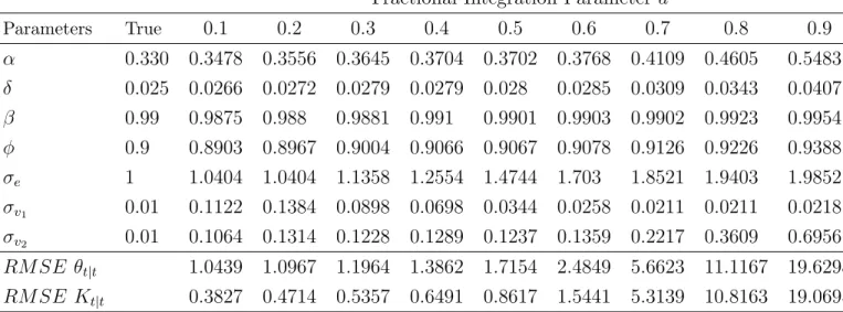
parameters and the implied dynamics for the state variables. Table one reports the simulation results and shows the true model parameters together with the mean of each estimated parameter for different degree of persistence. The last two rows report the Root Mean Square Error of the state variables (θt|tand Kt|t) predicted by

the Kalman filter.14

Fractional Integration Parameterd

Parameters True 0.1 0.2 0.3 0.4 0.5 0.6 0.7 0.8 0.9 α 0.330 0.3478 0.3556 0.3645 0.3704 0.3702 0.3768 0.4109 0.4605 0.5483 δ 0.025 0.0266 0.0272 0.0279 0.0279 0.028 0.0285 0.0309 0.0343 0.0407 β 0.99 0.9875 0.988 0.9881 0.991 0.9901 0.9903 0.9902 0.9923 0.9954 φ 0.9 0.8903 0.8967 0.9004 0.9066 0.9067 0.9078 0.9126 0.9226 0.9388 σe 1 1.0404 1.0404 1.1358 1.2554 1.4744 1.703 1.8521 1.9403 1.9852 σv1 0.01 0.1122 0.1384 0.0898 0.0698 0.0344 0.0258 0.0211 0.0211 0.0218 σv2 0.01 0.1064 0.1314 0.1228 0.1289 0.1237 0.1359 0.2217 0.3609 0.6956 RM SE θt|t 1.0439 1.0967 1.1964 1.3862 1.7154 2.4849 5.6623 11.1167 19.6298 RM SE Kt|t 0.3827 0.4714 0.5357 0.6491 0.8617 1.5441 5.3139 10.8163 19.0695

Table 1: Parameter estimation for different degrees of fractional integration d The bias tends to increase for all the model parameters as the persistence becomes stronger. For d bigger than 0.5, (Diebold and Rudebusch again) the bias becomes quite large especially for the capital share α, the capital depreciation δ and the variance of the productivity innovation σe: the estimated parameters are almost

twice as large as the true parameters. This is fairly consistent with what we find by comparing the estimates of the augmented and the standard filter on US data in the next section. In fact, although the “true” parameters used in the simulation can be considered to be close to the ones adopted in the calibration literature, the estimation with U.S. data produces values which are significantly higher and consistent with a parameter d larger than 0.5.

(20)

Finally the RMSE of the state prediction for both capital and productivity (last two rows of Table one) are very large. This is consistent with the large estimates of variances of the measurement errors σv1 and σv2. In fact, with a positive bias on

the variances of the measurement errors, the estimated Kalman gainK is lower than the true Kalman gain, producing consequently a prediction of the state which is too smooth and insensitive to innovations compared to the real state. This reflects the inability of the model to capture the true persistence of the data which is discharged as a noise component.

In Table 2 we report the results of the same exercise for the augmented filter.15

Fractional Integration Parameter d

Parameters True 0.1 0.2 0.3 0.4 0.5 0.6 0.7 0.8 0.9 α 0.330 0.3302 0.3301 0.3301 0.3299 0.3299 0.3299 0.3309 0.3342 0.3411 δ 0.025 0.025 0.025 0.025 0.0249 0.025 0.02499 0.0251 0.0253 0.0258 β 0.99 0.99 0.99 0.99 0.99 0.99 0.9900 0.99 0.9901 0.9903 φ 0.9 0.90 0.90 0.90 0.90 0.9 0.899 0.9002 0.9007 0.902 σe 1 0.9964 1.0017 1.0106 1.01 1.0295 1.0437 1.0598 1.0836 1.1301 σv1 0.01 0.0099 0.0099 0.0099 0.01 0.0099 0.0099 0.0099 0.0099 0.0099 σv2 0.01 0.0099 0.0099 0.0099 0.01 0.0099 0.0100 0.0119 0.0249 0.0524 RM SE θt|t 1.0154 1.0172 1.0342 1.0654 1.1241 1.2155 1.3512 2.6863 5.3401 RM SE Kt|t 0.2073 0.2542 0.3135 0.4014 0.5165 0.6899 0.9249 2.5774 5.1981 Table 2:

As it can be readily seen, the filter is able to estimate consistently the true parameters of the model. This is true for all the degree of fractional integration, even when the state variables become non-stationary (d > 0.5). Not surprisingly, the augmented filter provides much more accurate prediction of the underlying state variables compared to the standard filter. In fact, the RMSE errors of the state

15_{We choose a value of m, number of lags in productivity, equal to 30. This seems to be a}

reasonable compromise; while implementing a rather effective correction it does not exclude too many observations.

(21)

prediction are up to 4 times smaller than those obtained with the standard filter. This result is quite important and shows the ability of the modified filter to capture the dynamic properties of the data. As we show in the last section, this accuracy in predicting the data dynamics also holds when using the modified filter to forecast out-of-sample the observed variables.

4 Real data estimation

4.1 Model

In this section we take our model to the real data and repeat the Maximum Likelihood estimation of an RBC model as in Ireland (2004); the same type of model is also used by Ruge-Murcia (2007), in order to compare different estimation techniques. Households choose consumption and labour/leisure and save by investing in stocks of capital. Furthermore, they maximize the following utility function:

U0 =E0

∞

X

t=0

βt{log(ct) +γ(1−nt)}, (38)

subject to the budget constraint:

ct+it≤wtnt+rtkt−1,

there is no population growth and the total amount of labour is normalized to one and leisure is given by 1−nt. Capital accumulates with the standard law of

motion

ηkt= (1−δ)kt−1 +it, (39)

expressed in efficiency units in order to take into account a log-linear trend in technologyη. This gives rise to the (standard) first order conditions:

(22)

wt =γct (41)

The production function is given by the Cobb-Douglas:

yt=at(ηtnt)1−αktα−1, (42)

where technology evolves as:

log(at) = (1−ρ) log(ass) +ρlog(at−1) +t. (43)

In equilibrium the real interest rate equals the marginal productivity of capital minus the depreciation rate δ:

rt+δ=αatn1t−αk

α−1

t−1,

and the real wage rate equals the marginal productivity of labour:

wt = (1−α)atnαtkαt−1.

The model is closed by the market clearing condition:

yt =ct+it. (44)

The competitive equilibrium for the economy is the sequence of prices {rt, wt}∞0

and quantities {yt, kt, ct, nt, it}∞0 such that firms maximize profits, agents maximize

utility and all markets clear. The model is linearized by using the Taylor expansion of the system of equations (42), (40) (44),(43),(39),(41) around the steady state of the model. Then we solve the model following Klein (2000) and rewrite the reduced form solution into the (augmented) state space representation described in section 2. As before, we define withyt the vector of endogenous observable variables of the

model and withθtthe vector of unobservable exogenous processes. Following Ireland

(23)

measurement errors,ηt=

η_ty, η_tc, η_th 0

that are assumed to evolve as AR(1) processes

   η_ty η_tc ηh t   =    ρηy 0 0 0 ρηc 0 0 0 ρ_ηh       η_ty₋₁ η_tc−1 ηh t−1   +    ζ_ty ζ_tc ζh t    with E h ζ_t0ζt i =    σ2 ζy 0 0 0 σ2 ζc 0 0 0 σ2 ζh    .

Therefore we have yt = [yt, ct, ht] and θt= [kt, at, it, ηty, ηtc, ηth].

The following state space representation is then used to estimate the model:

θt+1 = Φθt+εt+1 yt=Hθt+vt where Φ = " pkk qka 0 _z # ; _z=       ρ 0 0 0 0 ρηy 0 0 0 0 ρηc 0 0 0 0 ρηh       H =    mck nca myk nya mrk nra   

where the elements of the matrices Φ and H are obtained from the solution of the model, i.e. for example:

(24)

ct =mckkt−1+ncaat.

In the presentation we focus only on one special treatment of measurement er-rors: three autocorrelated but mutually uncorrelated measurement errors. This is consistent with Ireland (2004) where he shows that such specification, compared with one having correlated measurement errors, have the best out-of sample forecasting properties in spite of less plausible values of the deep parameters. One of our claim is that this kind of trade off between forecasting and parameter estimation tend to vanish when long memory is taken into account.

Measurements are hours worked, consumption and GDP, which are taken re-spectively from BLS data (Current Employment Statistics) and US NIPA national accounting: data run from 1948:1 to 2002:2.16 _{We estimate the following set of}

structural parameters: α, η, γ, δ, ρ, ρηy, ρ_ηc, ρ_ηh, σ, σ_ζy, σ_ζc, σ_ζh plus the

level of technology ass which enters the steady state expressions of the variables. The estimated parameters are the capital share, the log-linear trend of technology, the parameter which pins down the amount of hours worked in steady state, the depreciation rate of capital, the persistence parameter of the technology and the measurement errors together with their standard deviations, and the discount pref-erence termβ. Differently from Ireland, we estimate the depreciation termδin order to show that long-memory correction can help in the identification of parameters that are sometimes found to be difficult to identify in the literature, and therefore they are calibrated.

4.2 Parameter estimates

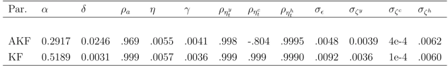
In this section we discuss the parameter estimates for two different models, AKF

refers to the augmented state space model, whileKF to the standard Kalman filter.

(25)

Par. α δ ρa η γ ρηy_t ρηc

t ρηht σ σζy σζc σζh

AKF 0.2917 0.0246 .969 .0055 .0041 .998 -.804 .9995 .0048 0.0039 4e-4 .0062 KF 0.5189 0.0031 .999 .0057 .0036 .999 .999 .9990 .0092 .0036 1e-4 .0060

Table 3: Parameter estimates

The estimation results differ substantially between the two filters17_{. Our finding}

suggests that there is a substantial amount of autocorrelation left over in the residuals

εt,which the standard Kalman filter does not account for, and consequently leads to

biased parameter estimates. From Table 3 we see that the share of capital estimated with the standard filter almost doubles the one given by the modified filter. There is a substantial difference in the values of both the persistence and variance parameters of the technology shock.

Overall, it seems that the augmented filter produces estimates which are in line with estimates produced by models with less restrictions on the variance-covariance matrices, such as the one with correlated shocks in Ireland (2004); moreover they are also closer to the values used in standard calibration exercises. Moreover there is a simple intuition explaining the large difference in estimated depreciation rates and capital shares. A large capital share and a low depreciation rate both make the policy function of capital more persistent. This happens both mechanically (less depreciation) and economically, since agents have more incentive, higher returns, to investing in capital goods. As a result the law of motion of capital in the reduced form of the model will have a stronger autoregressive term, i.e. it will be more persistent. Once data are cleaned from long memory, unexplained persistence does not bias estimates any longer.

(26)

5 Forecasting

In order to asses the ability of our approach to capture the dynamic properties of the data we compare the out of sample forecast of the modified filter with those of the standard Kalman filter. The ratio behind this exercise follows the results in Granger and Joyeux (1980) who showed that although it is always possible to find an AR representation that can adequately fit long memory dynamics, the forecast produced by such AR models will not be very accurate.

The exercise is implemented as follows. We estimate the RBC model described in the previous section with both the standard and our approach for a subsample of data, precisely from 1948:1 until 1987:4. We generate out-of-sample forecasts one through four quarters ahead for each variable and compare the root-mean-squared forecast errors from the modified model to those from the standard Kalman filter. We then extend the subsample by one period and repeat the estimation and forecasting. We continue this way until all the sample is covered in 2002.

Table 4 reports the RMSE together for the forecasts generated by the standard Kalman filter (KF) and those generated by the augmented filter (AKF). In order to asses whether any difference of the two RMSE is significant we also report the statistic proposed by Diebold and Mariano (1995).18

18_{The critical values for the Diebold and Mariano test have been obtained using a bootstrap}

(27)

Steps ahead 1 2 3 4 Output RMSE: AKF 0.6492 1.2294 1.8137 2.3585 RMSE: KF 0.984 1.8935 2.881 3.7871 D-M test -6.8582∗∗∗ -5.9845∗∗∗ -4.8295∗∗∗ -3.7659∗∗∗ Consumption RMSE: AKF 0.4588 0.7022 1.0155 1.3689 RMSE: KF 0.5443 0.961 1.4172 1.9213 D-M test -3.6916∗∗∗ -3.7701∗∗∗ -3.0075∗∗∗ -2.1948** Hours RMSE: AKF 0.6352 1.1373 1.6295 2.0847 RMSE: KF 0.8135 1.4583 2.0558 2.6461 D-M test -4.8812∗∗∗ -3.4673∗∗∗ -2.2781∗∗ -1.8388∗ Table 4:

The results indicate that forecasts from the modified filter significantly outper-form those from the standard Kalman filter. In particular, for output, the RMSE of the augmented filter are up to 60% smaller than those of the standard filter. This shows the better performance of the modified filter with respect to the normal one19. On one hand, the forecast from the augmented filter are more accurate than those from standard filter for all the steps ahead; on the other, the forecast accuracy of the modified filter improves, relatively to the standard filter, as the forecast horizon arises. This result indicates the presence of very persistent dynamics in the data that can not be fully captured by the autoregressive structure of the standard filter. On the other hand, it also shows that by accounting for such persistence it is possible to considerably improve the dynamic properties of the model.

(28)

6 Conclusion

In this paper we have shown a simple method to bring general equilibrium dynamic models to persistent data. This can be done by introducing one (or more) common factor long memory component as the driving forces of the data generating process. Existing techniques already allow researchers to estimate DSGE models under the assumption that data are either I(1) or I(0) with deterministic trend. In particular when data areI(1) it is possible to use a Diffuse Kalman filter under the assumption that the driving force of the economy such as technology is integrated of order one. This provides Maximum likelihood estimates of the deep parameters of the model under the assumption that there is a stochastic common trend.

A careful inspection of the data as well as relevant contributions to the economet-ric literature indicates that long memory is a relevant feature of real world economies. Long memory can be introduced in a general equilibrium framework by the aggre-gation of heterogeneous stochastic processes ,as in Abadir and Talmain (2002), at the price of having a very large and hard-to-handle framework. In this paper we take the shortcut of following the RBC thread by assuming that technology is it-self responsible for the long memory dynamic nature of the data. We believe to have good reasons for doing that since it is well documented by independent and methodologically different studies that productivity can have an I(d) nature.

We have shown that when unobservable states such as technology exhibit long range dependence, the standard Kalman filter approach to DSGE estimation is not well suited to tackle the estimation problem. In fact, the KF procedure can be summarized in two components: a state updating part and a signal extraction part (information set updating). Due to dynamic miss-specification, the direct updating of the states is incorrect; this generates a bias in the updating for the conditional variance of the unobservables. Due to the same miss-specification problem the or-thogonality condition between projected states and the innovations constructed by the filter fails to hold. This affects the signal extraction part and breaks down the op-timality of the recursive signal extraction method. We have found that the estimated deep parameters suffer of a bias; the estimation process and the filter incorrectly

(29)

in-troduces measurement error even when there is an almost zero measurement error in the data generating process.

We have proposed a method to take long memory into account. We view our procedure as a shortcut of the following assumption, that agents know the underlying dynamics of the economy and therefore their decision rules are correctly formed, still the econometrician cannot see individual shocks and its vision is corrupted by long memory and persistent autocorrelation. This informational assumption may be viewed as quite radical but we leave it to be relaxed in further research. Our work can also be viewed as a generalization of the methodology adopted in order to deal with trends: we filter the technology shocks in order to clean the state vector from long memory; this ensures that shocks are AR(1) with no more information left over in the residuals. The filtering technique we use is of a GLS type: we estimate the variance covariance matrix of the state vector, we factor its inverse by Cholesky decomposition and we use that to clean the state vector and to report it to anAR(1) with white noise.

Not only are the full sample estimates of our modified filter more in line with the calibration experience; we also show that in an out of sample forecasting exercise we outperform the conventional filter over all forecast horizons. This is due to the fact that we correctly take into account the autocorrelation of the data. Due to the flexible approach of Abadir and Talmain (2005) we evaluate the dynamic correlation of the state vector in such a way to be adequate even in the presence of a nonlinear autocorrelogram, while being able to approximate the (linear) fractional integration framework.

While we have applied our method to a simple RBC framework in principle there is no reason to be confined to such a unidimensional shock case. Several shocks can be accommodated in our framework. Nevertheless, as already said in the introduction, there is a widespread consensus about the I(d) nature of inflation; this would be a call for monetary and New Keynesian Models. Since these are mostly estimated by Bayesian Techniques we leave it to further research to extend our framework to that case.

(30)

References

[1] Abadir, K. M. and Talmain, G. (2002), “Aggregation, persistence and volatility in a macromodel”, Review of Economic Studies, 69, 749-779.

[2] Abadir, K. M. and Talmain, G. (2005), “Distilling co-movements from persis-tence macro and financial series”, ECB working paper no. 525.

[3] Abadir, K. M., Caggiano, G. and Talmain, G. (2006),“ Nelson and Plosser revised: the ACF approach”, working paper 2005-7, University of Glasgow. [4] Altissimo, F., Mojon, B., Zaffaroni, P. (2005), “Fast micro and slow macro: can

aggregation explain the persistence of inflation?”, ECB Inflation Persistence Network Paper.

[5] Carvalho, C. (2006). ”Heterogeneity in Price Stickiness and the Real Effects of Monetary Shocks”, The B.E. Journal of Macroeconomics: Vol. 2 : Iss. 1 (Frontiers)

[6] Chamber, M.J. (1998). ”Long memory and aggregation in Macroeconomic time series”, International EConomic Review, 39 (4), 1053-1072

[7] Diebold, F. X. and Rudebusch, G. D. (1989), ”Long memory and persistence in aggregate output”, Journal of Monetary Economics, vol. 24(2), 189-209.

[8] Durbin, J. and Koopman, S.J. (2001), ”Time series analysis by state space methods”, Oxford University Press.

[9] Gadea, M.and Mayoral, L. (2006), ”The Persistence of Inflation in OECD Coun-tries: A Fractionally Integrated Approach,” International Journal of Central Banking, vol. 2(1).

[10] Granger, C. W. J. (1980), “Long memory relationship and the aggregation of dynamic models”, Journal of Econometrics, 14, 227-238.

(31)

[11] Granger, C. W. J. and Joyeux, R. (1980), An introduction to long-memory time series models and fractional differencing, Journal of Time Series Analysis 1, 15-30.

[12] Hamilton, J. (1994), Time Series Analysis. Princeton University Press.

[13] Ireland, P. (2004), ”A method for taking models to the data,” Journal of Eco-nomic Dynamics and Control, vol. 28(6), pages 1205-1226.

[14] Mayoral, L. (2005).,”Further evidence on the statistical properties of Real GNP,” Economics Working Papers 955, Department of Economics and Business, Uni-versitat Pompeu Fabra, revised Feb 2006.

[15] McGrattan, E. (2007), ”Measurement with Minimal Theory,” 2006 Meeting Pa-pers 338, Society for Economic Dynamics

[16] McGrattan, E. (1994), ”The macroeconomic effects of distortionary taxation,” Journal of Monetary Economics, Elsevier, vol. 33(3), 573-601.

[17] Moretti, G. (2007), ”Detecting long memory co-movements in macroeconomic time series”, Bank of Italy working paper 642.

[18] Ravenna, F. (2007), ”Vector Autoregressions and Reduced Form Representa-tions of DSGE models” Journal of monetary economics, Vol. 54 N. 7

[19] Robinson, P. (2003), Time Series with long memory. Oxford University Press. [20] Ruge-Murcia, F. J. (2007). ”Methods to estimate dynamic stochastic general

equilibrium models,” Journal of Economic Dynamics and Control, vol. 31(8), 2599-2636.

[21] Sowell, F. (1992), “Modeling long-run behavior with the fractional ARIMA model”, Journal of Monetary Economics 29, 277-302.

(32)

Département des Sciences Économiques de l'Université catholique de Louvain Institut de Recherches Économiques et Sociales

Place Montesquieu, 3 1348 Louvain-la-Neuve, Belgique