Performance evaluation of network processor architectures: combining simulation with analytical estimation

(1)

Performance evaluation of network processor architectures:

combining simulation with analytical estimation

Samarjit Chakraborty

a,*

, Simon K€

u

unzli

a

, Lothar Thiele

a

,

Andreas Herkersdorf

b

, Patricia Sagmeister

b

a_{Computer Engineering and Networks Laboratory, Swiss Federal Institute of Technology (ETH) Z}_€

u

urich, Gloriastrasse 35, CH-8092 Z€uurich, Switzerland

b_{IBM Zurich Research Laboratory, S}_€_a_a_{umerstrasse 4, CH-8803 R}_€_u_u_{schlilion, Switzerland}

Abstract

The designs of most systems-on-a-chip (SoC) architectures rely on simulation as a means for performance estimation. Such designs usually start with a parameterizable template architecture, and the design space exploration is restricted to identifying the suitable parameters for all the architectural components. However, in the case of heterogeneous SoC architectures such as network processors the design space exploration also involves a combinatorial aspect––which architectural components are to be chosen, how should they be interconnected, task mapping decisions––thereby in-creasing the design space. Moreover, in the case of network processor architectures there is also an associated uncer-tainty in terms of the application scenario and the traffic it will be required to process. As a result, simulation is no longer a feasible option for evaluating such architectures in any automated or semi-automated design space exploration process due to the high simulation times involved. To address this problem, in this paper we hypothesize that the design space exploration for network processors should be separated into multiple stages, each having a different level of abstraction. Further, it would be appropriate to use analytical evaluation frameworks during the initial stages and resort to simulation techniques only when a relatively small set of potential architectures is identified. None of the known performance evaluation methods for network processors have been positioned from this perspective.

We show that there are already suitable analytical models for network processor performance evaluation which may be used to support our hypothesis. To this end, we choose a reference system-level model of a network processor ar-chitecture and compare its performance evaluation results derived using a known analytical model [Thiele et al., Design space exploration of network processor architectures, in: Proc. 1st Workshop on Network Processors, Cambridge, MA, February 2002; Thiele et al., A framework for evaluating design tradeoﬀs in packet processing architectures, in: Proc. 39th Design Automation Conference (DAC), New Orleans, USA, ACM Press, 2002] with the results derived by detailed simulation. Based on this comparison, we propose a scheme for the design space exploration of network processor ar-chitectures where both analytical performance evaluation techniques and simulation techniques have unique roles to play.

Keywords:Performance analysis; Network processors; High-performance routers; Application-speciﬁc instruction set processors

*

Corresponding author.

E-mail addresses:[email protected](S. Chakraborty), [email protected] (S. K€uunzli), [email protected] (L. Thiele), [email protected] (A. Herkersdorf), [email protected] (P. Sagmeister).

(2)

1. Introduction

Today, network processors play an important role in the design of modern routers. Therefore, of late there has been a lot of interest in the study of network processor architectures. Designing such architectures is partly complicated by the fact that they involve complex tradeoffs between flexibility and efficiency. Typically, such processors are re-quired to process packets at high line speeds, support complex packet processing functions, and to a large extent be programmable to incorporate new functionality. To support such stringent and to some extent conflicting demands, most network processors available today consist of a collection of heterogeneous processing elements, memory subsystems and on-chip communication

infra-structure. There is no agreement on a generic

net-work processor architecture and a wide variation exists among the processors available in the mar-ket today. However, typically they are built around one or more processor cores and micro-engines, some dedicated hardware for packet processing tasks such as header parsing, table lookup, etc., some on-chip cache/memory, and specialized buses and bridges for on-chip communication and in-terfacing with external memories and ports.

Because of these new and different require-ments, designing and evaluating a network pro-cessor architecture calls for specialized modeling techniques and frameworks which do not fall under the preview of traditional embedded pro-cessor design. As a result, recently there has been a number of proposals for performance models and design frameworks specific to network processor architectures (see [6,7,9,26,27,31,32]). The goal of these frameworks and models is to aid a designer in understanding the performance tradeoffs in-volved in a design and come up with an optimal architecture that suits the application scenario at hand.

Realizing these goals in the context of tradi-tional embedded processor design typically in-volves a method for performance evaluation of the architecture, and a means for automatic design space exploration. In most of these cases it is

possible to formulate a parameterizedarchitecture

template, where the design space exploration is

restricted to finding appropriate values of the pa-rameters such as bus width, cache associativity and cache size. The resulting design space is therefore reasonably small and it is usually feasible to ex-haustively evaluate all the possible designs by simulation. In cases where the design space is rel-atively larger, techniques such as partitioning the architecture into disjoint subsystems and using independent design space explorations for the different subsystems have been used [11,15,22]. Even in these cases, the choice of the different ar-chitectural components is usually fixed (for ex-ample, see [1,24], where the system always consists of a VLIW processor, a systolic array and a cache subsystem and the design space exploration con-sists of identifying appropriate parameters for each of these components), and there are no un-certainties associated with the application, as is the case with network processor architectures. 1.1. Network processor design

In the case of network processor design, the issue of design space exploration, however, might have a different complexity because of several reasons. Network processor architectures are very heterogeneous in nature and usually it is not pos-sible to define a parameterizable template archi-tecture. As a result the design space is larger compared to those in the case of typical embedded processor architectures and involves a combina-torial aspect in addition to traversing the para-meter spaces of the different components. These processors might also be used in multiple appli-cation scenarios (such as core or access networks), might be required to support different traffic classes (where some classes might have quality-of-service requirements and others have minimum throughput requirements), and at the same time should be flexible to be able to incorporate new functionality. In order to account for all of these issues in the design phase, we believe that new design methodologies are required. In particular, resorting to exhaustive simulations of all possible designs will no longer be a feasible option for au-tomated design space exploration. Hence, using other means of performance evaluation such as analytical models is necessary.

(3)

It is known that typically the design ﬂow of complex systems-on-a-chip (SoC) architectures starts with an abstract description of the applica-tion and some performance requirements, which are then used to drive a system-level design space exploration for identifying a suitable architecture. This involves evaluating many prospective archi-tectures on a system-level and an iteration loop between the exploration and the evaluation steps. Once the main architectural decisions have been made, the resulting architectures are then more accurately evaluated, possibly on the basis of many other criteria which were not considered previously. The design space exploration at this stage, in contrast to the previous, might only in-volve tuning the parameters of diﬀerent cores in a core-based SoC design.

1.1.1. Our contributions and relation to previous work

In this paper we argue that in the case of het-erogeneous SoC architectures, this separation of the design space exploration into multiple stages is all the more important in order to tackle the large and the diﬀerent nature of the design space. In particular, we hypothesize that in the context of network processors, the underlying framework for performance evaluation should vary depending on the stage of the design space exploration––it will be more appropriate to use analytical methods during the initial stages and resort to simulation when a relatively small set of promising alterna-tives has been identiﬁed. None of the known per-formance evaluation frameworks for network processors have been evaluated or positioned from

this perspective. From a designerÕs point of view it

would be useful to know if any of the known modeling techniques are more suitable for a par-ticular stage of the architecture design.

In any of the design phases, for a potential ar-chitecture at hand, the performance evaluation needs to answer questions such as: Does this ar-chitecture meet the required line speeds and max-imum allowable delays experienced by packets? What are the limits to the improvement in pro-cessor or bus utilization as the number of proces-sor cores is increased? How does the cache/ memory organization impact these limits? Will a

given hardware assist improve the system perfor-mance compared to a software implementation? We believe that the exact nature of these questions, how accurately they need to be answered, and what is the allowable computation/simulation time required to answer them strongly depend on the design phase. For network processors many of these can be adequately answered with a system-level model, and we show that there exist suitable analytical frameworks for doing this. These are orders of magnitude faster when compared to simulations and are hence appropriate for a sys-tem-level design space exploration where the de-sign space can be very large.

In support of our hypothesis, we compare the results obtained by a system-level analytical per-formance model proposed in [26,27] with detailed cycle accurate simulations, on a realistic network processor architecture. We consider three perfor-mance metrics: (i) the line speed or the end-to-end throughput that can be supported by the archi-tecture, which is measured using the utilization of its diﬀerent components (processors, buses) and thereby also identifying which component acts as the bottleneck, (ii) the end-to-end packet latencies, and (iii) the on-chip cache/memory requirement of the architecture. Many important questions that arise in the context of network processor archi-tectures pertain to these metrics. The usefulness of the results obtained from the analytical model should be evaluated with respect to their relative accuracy when compared to the simulation results, and the time it takes to compute these results compared to simulation times (under the assump-tion that there is a high conﬁdence in the simula-tion results).

One of the major criticisms of the analytical framework [26,27] we consider here, has been that although it is suﬃciently general, it still remains to be seen if it can be applied to analyse any realistic network processor architecture (see, for example, [29]). Our work in this paper addresses this issue and additionally places this framework in an ap-propriate stage of the design ﬂow.

In the next section we review the existing modeling techniques known for network processor performance evaluation. For the sake of complete-ness, we present the analytical model considered in

(4)

this paper in Sections 3 and 4. In Section 5 we describe the setup used for the simulation. A comparison of the results obtained by the two methods on a reference architecture is made in Section 6. Finally, in Section 7 the results of the comparative study are analysed, and on the basis of these results we propose a methodology for the design space exploration of network processor architectures which relies on both the compared techniques.

2. Existing approaches

As mentioned in the last section, lately there has been a number of proposals for performance analysis techniques specific to network processor architectures––both analytical models and simu-lation based frameworks. There is also a large body of work devoted to system-level performance evaluation of SoC architectures (see [10] and the references therein) and also of more specific aspects of an architecture such as the on-chip communication infrastructure (see [17] and the references therein). However, in this section we focus on the work done specifically in the context of network processors.

In [6] a modeling framework is presented which is composed of independent application, system and traﬃc models. The application is modeled using the Click modular router from MIT[16]. Click consists of a collection of software modules for describing various router functionalities. Such

modules in Click are calledelements, and by

put-ting together diﬀerent elements in the form of a

graph (which is called aconﬁguration) it is possible

to construct IP routers, firewalls, QoS routers, etc. The framework in [6] is based on compiling Click modules for the Alpha ISA [3]. The archi-tecture to be evaluated is simulated using Simpl-eScalar [5] and it implements the Alpha instruction set. The compiled Click modules are then executed on this architecture. By simulating this execution using different traffic traces, the profiled code yields various information such as instruction count, details regarding cache behavior, etc. These are then used to compute various performance metrics for the architecture being evaluated,

re-lated to packet latency, bandwidth and resource utilization. For elements which do not have any software implementation (such as dedicated hard-ware units for header parsing) and cannot be sim-ulated, the proﬁle and external dependencies need to be provided manually by the user.

In contrast to this approach, the work done in [32] models an architecture in SystemC [12]. This work mostly focuses on the communication sub-system and the memory organization of an archi-tecture. The models are then simulated on packet traces and performance metrics such as bus utili-zation, memory ﬁll levels, and packet delays are evaluated. This work forms the basis of the sim-ulations results that we present in this paper and further details on it are given in Section 5.

These two approaches as they exist now are complementary to each other. Crowley and Baer [6] use an accurate processor model but a very ele-mentary model of the communication subsystem of an architecture (such as buses, bridges, etc.). On the other hand, the framework in [32] implements cycle accurate models for buses and bridges, but has a very simple processor and application model. Clearly, there exists an opportunity to combine the above frameworks which will then consist of a detailed model of processors as well as other components of the communication subsystem, such as buses, for which SystemC models already exist. Additionally, in the same way as there exists a SimpleScalar model of the Alpha processor, there already exists a SystemC model of PowerPC which can be simulated on executable code. This easily opens the opportunity of integrating this model into the network processor architecture model and have detailed applications models, as for example is done in [6] using Click.

An analytical performance model of a network processor is considered in [9]. Here the diﬀerent components that make up the architecture, and the interconnection among these components (the so

called architecture template) is ﬁxed. The design

decisions that are to be made in deriving a concrete architecture from such a template, consist of choosing the values of the various parameters such as the bus width, cache sizes, etc. The architecture considered consist of a number of multithreaded processors organized in clusters. Each cluster

(5)

con-sists of a number of processors, each having its own cache, and the cluster communicates with an oﬀ-chip memory using its own memory interface. The parameters that can be changed are the number of threads running in each processor, the cache sizes, the number of processors in each cluster, the number of clusters in the network processor, the width of the memory channels, etc. For evaluating a set of parameters, an analytical model for multithreaded processors proposed by Agarwal [2] is used. Most of this work can be viewed as a model for the cache/memory subsys-tem of a network processor architecture. The an-alytical model is then evaluated on a benchmark workload [30] consisting of a mix of header-processing and payload-header-processing applications. For each application, properties such as load and store instruction frequencies and instruction and data cache miss rates are measured using processor and cache simulators. These values are then used to evaluate an architecture in terms of its pro-cessing power per unit chip area. This model can therefore be viewed as a combination of analytical methods and simulation, and might be restrictive for use in a fast design space exploration method because of the simulation times involved.

The analytical model [26,27] used for the com-parative study in this paper uses a model for both the architecture and the traffic traces on which the architecture is evaluated. In contrast to the work in [9] the architecture layout or the topology in this case is not fixed. Therefore, different combinations of processors, buses and their interconnection can be modeled and evaluated. The details of this model are presented in the next two sections.

3. A model for characterizing network traﬃc and packet processing resources

In this section we describe a model for charac-terizing packet ﬂows, and based on similar con-cepts, a model for describing the computation/ communication power of resources used to pro-cess/transmit the packets entering a resource.

These models are based on the concept ofarrival

andservicecurves due to Cruz [8], and Parekh and Gallager [19].

Let f be a ﬂow entering a given resource. The

resource is either a computation resource such as a processor on which some packet processing task is implemented, or it is a communication resource such as a bus that is used to transmit packets be-tween two computation resources or a

computa-tion resource and a memory module. Let RfðtÞ

denote the number of packets from f arriving at

the resource during the time interval ½0;t. T he

maximum number of packets arriving at the re-source is assumed to be bounded by a

right-con-tinuous subadditive function called the upper

arrival curve denoted by au

f. Similarly, a lower

bound on the number of packets arriving at the

resource is given by a lower arrival curvedenoted

byal

f.a l f anda

u

f together can be referred to as the

traﬃc constraint functions and they satisfy the following inequality: al fðtsÞ6RfðtÞ RfðsÞ6aufðtsÞ; 806s6t: For any DP0,al fðDÞP0 anda l fð0Þ ¼a u fð0Þ ¼0. Therefore, al

fðDÞ gives a lower bound on the

number of packets that can arrive at the resource

from the ﬂowf within any time interval of length

D.au

fðDÞgives the corresponding upper bound.

Similar to the arrival curves describing packet ﬂows, the computation or communication

capa-bility of a resource is described using service

curves. Given a resource r, let CrðtÞ denote the number of packets (or the number of bytes, de-pending on the resource) that can be processed by

rduring the time interval½0;t. Then the upper and

lower service curvesbu_r andbl_r describing the

pro-cessing capabilities of the resource satisfy the fol-lowing inequality:

bl_rðtsÞ6_C_r_ð_t_Þ_C_r_ð_s_Þ6_bu

rðtsÞ; 806s6t:

Further, for any DP0, bl_rðDÞP0 and bl_rð0Þ ¼

bu_rð0Þ ¼0. Therefore, bl_rðDÞ is a lower bound on

the number of packets that can be processed byr

(or the number of bytes that can be transmitted in

case r is a communication resource) within any

time interval of length D. Likewise, bu_rðDÞ is the

corresponding upper bound. Hence, the processing

capability ofrover any time interval of lengthDis

always greater than or equal tobl_rðDÞand less than

(6)

As mentioned above, the arrival curves of a

ﬂowf entering a resourceris described in terms of

either the number of bytes entering r within any

time interval of lengthDor the number of packets

within any time interval of lengthD. This depends

on the packet processing task implemented on r.

For a task such as packet header processing, where

the load on r depends on the number of packets

entering and not on the sizes of the packets, the arrival curves are deﬁned in terms of number of

packets. On the other hand, if r is a

communica-tion resource such as a bus, or a payload pro-cessing task such as encryption is implemented on

r, then the arrival curves are deﬁned in terms of

number of bytes.

Now suppose that for each packet (or each

byte, as the case maybe) entering the resourcer,w

units of processing resource have to be spent byr

to process the packet. This might be described as the number of processor cycles, bus cycles, or

processor instructions. Then if a ﬂowf has arrival

curves aal

f andaauf described in terms of number of

packets, these maybe transformed as follows to

represent the processing request demanded by f

from the resourcer:

al_f ¼waal_f; au_f ¼waau_f:

Hence, al

f and a u

f now describe the arrival

curves of ﬂowf in terms of the processing request

(for example, number of processor cycles)

de-manded from r. If bl_r and bu_r describe the

pro-cessing capability of r in terms of the same units

(i.e., processor cycles) then the maximum delay and maximum backlog suﬀered by packets of ﬂow

f at the resource r can be given by the following

inequalities: delay6_sup tP0 infns n P0:au_fðtÞ6_bl rðtþsÞ oo ; ð1Þ backlog6_sup tP0 au_fðtÞ n bl_rðtÞo: ð2Þ

A physical interpretation of these inequalities can be given as follows: the delay experienced by

packets waiting to be served byrcan be bounded

by the maximum horizontal distance between the

curves au

f andb l

r, and the backlog is bounded by

the maximum vertical distance between them.

The packets of ﬂowf, after being processed by

the resourcer, emerge out of this resource. Letau0

f

and al0

f be the upper and lower arrival curves of

this processed ﬂow. Similarly, letbu_r0andbl_r0 be the

upper and lower remaining service curves of the

resource r, denoting the remaining processing

ca-pability of r after processing packets of ﬂow f.

Then these can be given as follows (see [28] for further details and proofs):

al_f0ðDÞ ¼ inf 06t6D a l fðtÞ n þbl_rðDtÞo; ð3Þ au0 fðDÞ ¼₀₆inf_t₆_D sup vP0 au fðt n þvÞ bl_rðvÞo þbu_rðDtÞ;bu_rðDÞ ; ð4Þ bl_r0ðDÞ ¼ sup 06t6D bl_rðtÞ n au_fðtÞo; ð5Þ bu_r0ðDÞ ¼ sup 06t6D bu_rðtÞ n al_fðtÞo: ð6Þ

The maximum utilization of the resourcer due

to the processing of ﬂowf is given by

utilization6 _lim

D!1

bu_rðDÞ bl_r0ðDÞ

bu_rðDÞ : ð7Þ

4. An analytical model for network processor performance evaluation

The modeling concepts used in the last section are known from work done in the area of com-munication networks. The results derived on the basis of these models (see also [28]) have their background in network calculus [4] which use the concept of arrival and service curves in a network theoretic context. In this section we show how these results can be used to formulate an analytical performance evaluation model for network pro-cessors. The results here were originally derived in [26,27] and we refer the reader to these papers for additional details.

Here we view a network processor as a collec-tion of diﬀerent processing elements (such as CPU

(7)

cores, micro-engines, and dedicated units like hardware classifier, cipher, etc.) and memory modules connected to each other by communica-tion buses. On each of these processing elements one or more packet processing tasks are imple-mented. Depending on the sequence in which these tasks process a packet, and the mapping of these tasks onto the different processing elements of the network processor, any packet entering the network processor follows a specific sequence through the different processing elements. The flow to which this packet belongs is associated with its arrival curves. Similarly all the resources have their associated service curves. As the packets of the flow move from one processing element to the next, and also cross communication resources such as buses, both, the arrival curves of the flow and the service curves of the resources get modified following the Eqs. (3)–(6) given in Section 3. Given this, the maximum end-to-end delay experienced by any packet, the on-chip memory requirement of the network processor, and the utilization of the different resources (both computation and com-munication) can now be computed using Eqs. (1), (2) and (7).

To formally state the above procedure, consider

that for the set of ﬂows F entering the network

processor, there is a task graph G¼ ðV;EÞ. Any

vertex v2V denotes a packet processing (or

communication) task. For any ﬂow f 2F, let

VðfÞ V denote the set of packet processing tasks

that have to be implemented on any packet from

F. Additionally, a subset of directed edges fromE

deﬁnes the order in which the tasks inVðfÞshould

be implemented on any packet fromf. Therefore,

ifu,v2VðfÞrepresent two tasks such that for any

packet belonging to f, the task v should be

im-plemented immediately after task u, then the

di-rected edgeðu;vÞbelongs to the setE. Hence, for

each ﬂow f there is a unique path through the

graph G starting from one of its source vertices

and ending at one of its sink vertices. The vertices on this path represent the packet processing tasks

that are to be implemented on packets fromf.

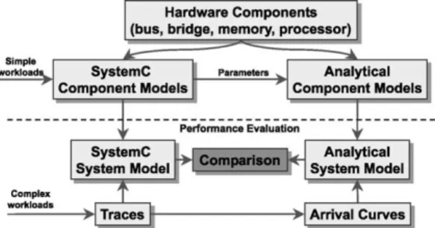
Fig. 1 shows a hypothetical network processor architecture built out of blocks from an existing core library [13,14]. Here PPC refers to the Power-PC 440 core, and PLB and OPB refer to two buses

called the processor local bus and the on-chip peripheral bus provided by the CoreConnect [14] architecture for interconnecting cores and custom logic. The numbers on the arrows in this figure indicate actions that are to be performed by the different blocks as a packet flows through the ar-chitecture, and they are ordered according to the numbering.

From Fig. 1 it is possible to construct a task graph considering the appropriate packet transfers from one resource to another. This task graph can then be used to compute the load on the diﬀerent buses (such as the OPB and the PLB), the on-chip memory requirement of this architecture to store the buﬀered packets in front of each resource, and the end-to-end packet delays.

4.1. Analysis using a scheduling network

In Section 3 we described how to compute the delay and backlog experienced by a flow passing through a single resource node processing the flow. For this we characterized the flow using its arrival curves and the resource node using its service curves and also derived formulas for the maximum utilization of this resource and the outgoing arrival and resource curves. Now we extend these results

Fig. 1. A system-level model of a network processor. The ﬁgure shows the path that a packet follows through the architecture. The numbers on the arrows indicate the diﬀerent actions in-volved (which are explained in Table 1) while the packet travels through the architecture, and specify the order in which these actions are executed. Further details of this model can be found in Section 6.

(8)

to consider the case where the ﬂow passes through multiple resource nodes as shown in Fig. 1.

The outgoing arrival curve captures the char-acteristics of the processed packet flow (for ex-ample its burstiness and long-term rate), which might be different from the characteristics the flow has before entering the resource. Similarly the outgoing service curve indicates the remaining processing capability of the resource after pro-cessing the flow. The idea now is to use this out-going arrival curve as an input to another resource node (more precisely, the resource node where the next packet processing task, as given by task graph described above, is implemented). In the same way, the outgoing service curve of the first re-source is used to process packets from a possibly second flow. This procedure can be illustrated

using a scheduling network. For example, Fig. 2

shows the scheduling network corresponding to the packet traversal through the architecture shown in Fig. 1.

In general, multiple flows enter a network pro-cessor and are processed by the different resources in the order specified by the task graph described above. As packets from several flows arrive at a resource, they are served in an order determined by the scheduling policy implemented at the

re-source. For example, many buses use a fixed pri-ority bus arbitration scheme. Other scheduling policies might be first-come-first-serve (FCFS) and round robin. Here, we illustrate the analytical model assuming that all the resources use fixed priority. However, the model can be extended to incorporate other scheduling policies as well.

Let us assume that there are n ﬂows f1;. . .;fn

arriving at a resourcer, which serves these ﬂows in

the order of decreasing priorities, i.e., f1 has the

highest priority andfnthe lowest. For each packet

of the ﬂowfi, some packet processing task ti

im-plemented on resourcerprocesses the packet and

this requires wðti;rÞ processing units from r. For

example,wðti;rÞmight be the number of processor

instructions, or bus cycles in case r is a

commu-nication resource. We henceforth denotewðti;rÞby

wi when it is clear which resource is being

re-ferred to. Each ﬂow fi arriving at r is

associ-ated with its upper and lower arrival curves aau

i

and aal

i respectively and receives a service from r

which can be bounded by the upper and lower

service curves bu_i and bl_i respectively. The service

available fromrin the unloaded state (i.e., before

any of the ﬂows f1;. . .;fn are served) is bounded

by the upper and lower service curves bu and bl

respectively.

in OPB

target resource nodes(output service curves),

used to compute remaining processing/communication capability

source resource nodes(input service curves)

in

out

source and target packet nodes

input arrival curves (derived from traces)

final ouput arrival curves PLB read in out Get BD Transfer Packet to Memory Get Buffer-Descriptor (BD) PLB write in out Transfer Packet to Memory out Transfer Packet Header Store Modified Packet Header Get BD Transfer Packet to EMAC Transfer Packet to EMAC Memory Status Update

(9)

In the fixed priority scheme,rserves the flows in the order of decreasing priorities and the remain-ing service curve after processremain-ing a flow is used to serve the lower priority flows. The resulting arrival curves and the remaining service curves can be computed using Eqs. (3)–(6) given in Section 3. Since packets from different flows might have

dif-ferent processing requirements given byw1;. . .;wn,

the arrival curves ﬁrst need to be scaled as de-scribed in Section 3. Similarly, the outgoing arrival

curves need to be scaled back as follows. Ifau0

i and

al0

i are the outgoing arrival curves from a resource

node calculated using Eqs. (3) and (4), then a au0 i ¼ da u0 i =wie and aal 0 i ¼ ba l0 i=wic. The ﬂoor/ceiling

functions are used since a subsequent resource node can start processing a packet only after the

task implemented onrﬁnishes processing it.

Finally, given the service curves for the

un-loaded resource bu and bl, and the arrival curves

a au

i,aa l

i,i¼1;. . .;n, we show how the service curves

bu_i and bl_i for i¼1;. . .;n can be determined. As described before, au_i ¼wiaaui; a l i¼wiaali; i¼1;. . .;n; a au0 i ¼ da u0 i=wie; aal 0 i ¼ ba l0 i=wic; i¼1;. . .;n; bu₁ ¼bu; bl₁¼bl; bu_i ¼bu_i0₁; bl_i¼bl_i0₁; i¼2;. . .;n;

wherebu_i0₁ andb_il0₁fori¼2;. . .;nare determined

frombu_i₁,bl_i₁,au

i1 anda l

i1 by applying Eqs. (5)

and (6) from Section 3. Lastly, the remaining ser-vice curve after processing all the ﬂows is given as follows:

bu0 ¼bu_n0; bl0 ¼bl_n0:

These can be used to compute the maximum uti-lization of the resource using the inequality (7). The processed ﬂows with their resulting arrival

curves aau0

i andaa l0

i now enter other resource nodes

for further processing.

4.2. Scheduling network construction

Using the results in the last section we now describe the procedure for constructing a sched-uling network. This can then be used to determine properties of the architecture such as the on-chip

memory requirement, the end-to-end delay expe-rienced by packets and the utilization of the dif-ferent on-chip resources such as processors and buses.

The inputs necessary for constructing such a network are the task graph which denotes for each ﬂow the sequence of packet processing tasks that are to be executed on any packet of the ﬂow and the target architecture on which these tasks are mapped.

The scheduling network contains one source

resource nodeand onetarget resource nodefor each resource used in the architecture. Similarly, for

each packet ﬂow there is asource packet nodeand

a target packet node. For each packet processing task of a ﬂow there is a node in the network marked with the task and the resource on which this task is implemented. For two consecutive

tasks u and vof a ﬂow, if u is implemented on a

resource ruandvon a resourcerv then there is an

edge (drawn horizontally in the Fig. 2) in the

scheduling network from the nodeðu;ruÞtoðv;rvÞ.

For a given ﬂow, if u and vare two tasks

imple-mented on the same resourceranduprecedesvin

the task graph, then there is an edge (drawn

ver-tically in the Fig. 2) from the node ðu;rÞ to the

node ðv;rÞ.

The arrival curves of the ﬂows and the service curves of the resources pass from one node to the next in the scheduling network and get modiﬁed in the process, following Eqs. (3)–(6).

For a given ﬂow f, let au

f be its upper arrival

curve before entering the network processor. Suppose this ﬂow passes through nodes of the scheduling network which have their input lower

service curves equal to bl₁;. . .;bl_m. Then the

accu-mulated lower service curve bl used to serve this ﬂow can be computed as follows:

b bl₁¼bl₁; b bl_i_þ₁¼ inf 06t6D b bl_iðtÞ n þbl_i_þ₁ðDtÞo; i¼2;. . .;m1; bl¼bbl_m:

Now the maximum end-to-end delay and the total backlog experienced by packets from the ﬂow

(10)

delay6_sup tP0 infns n P0:au_fðtÞ6_bl_ð_t_þ_s_Þ oo ; ð8Þ backlog6_sup tP0 au fðtÞ n blðtÞo: ð9Þ

Compared to independently deriving the delay and backlog at single resources using inequalities (1) and (2) from Section 3 and adding them, the inequalities (8) and (9) give tighter bounds. 4.3. Approximating the arrival and service curves

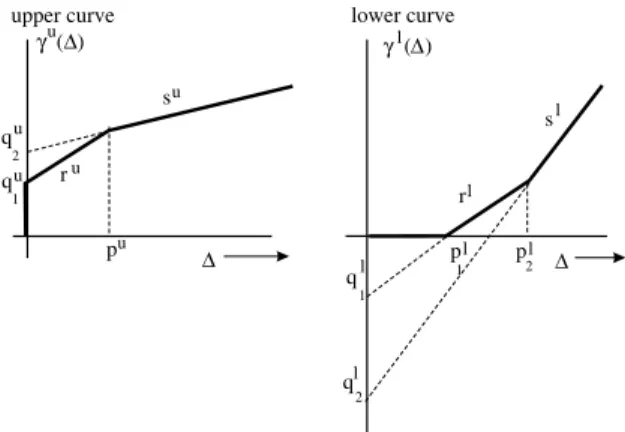
The Eqs. (3)–(6) are clearly expensive to com-pute for general arrival and service curves. More-over, these equations need to be computed for all the nodes of a scheduling network. Additionally, if these curves are to be meaningfully derived out of packet traces (as shown later in this paper), then the resulting curves can be described by a few parameters such as the maximum packet size, the short-term burst rate, and the long-term packet arrival rate. In view of this, we propose a piecewise linear approximation of all arrival and service curves. Using these approximations, the Eqs. (3)– (6) can be eﬃciently computed, thereby avoiding the computational bottleneck involved in dealing with general curves.

Each curve in this case is approximated using a combination of three straight line segments. This allows us to exactly model an arrival curve in the form of a T-SPEC [23], which is widely used in the area of communication networks. Fig. 3 shows

the resulting form of the upper and lower curves

(both arrival and service). Here qu

1 represents the

maximum possible load on a resource for

pro-cessing one packet. The slope ru _{of the middle}

segment of the upper curve can be interpreted as

the burst rate, and the slopesu _{as the (load on a}

resource due to the) long-term packet arrival rate.

In the case of communication resources, qu

1

rep-resents the maximum packet size. The values ofpu

andpl

1,p l

2can be computed from these parameters.

Any upper (saycu_{) and lower (say}_cl_{) curves can}

now be written as the following:

cu_ð_D_{Þ ¼}_min _qu 1 þruD;qu₂þsuD; clðDÞ ¼maxql₂þslD;ql₁þrlD;0; where qu 2Pq u 1P0; r u_P_su_P₀_; _ru _¼_su₍₎_qu 1 ¼q u 2; ql 26q l 160; 06r l₆_sl_; _rl_¼_sl₍₎_ql 1¼q l 2: Using these curves, the Eqs. (3)–(6) as well as maximum delay and backlog can be evaluated ef-ﬁciently using symbolic techniques.

5. The simulation setup

Even in cases where analytical models exist, performance evaluation of processor architectures using simulation still continues to be the most widely used procedure. This is primarily motivated by the accuracy of the results that can be obtained using simulation, and the second reason being ﬂexibility. In many cases analytical models cannot capture all the aspects of an architecture and are often restricted to one particular level of abstrac-tion.

In this section we outline the methodology for model composition and performance evaluation of network processor architectures based on simula-tion, which forms the basis for comparing the re-sults obtained from the analytical framework presented in the last two sections. This section is based on the work presented in [32] and more detailed explanations concerning the models can be found there. Here the primary goal is to illus-trate the abstraction level at which the diﬀerent components of the architecture are modeled.

Sec-upper curve γ ∆u( ) l( ) ∆ r s p lower curve ∆ r s q p u u u l l l l qu 2 qu 1 1 ql 2 1 pl 2 γ ∆

Fig. 3. Piecewise linear approximations of the upper and lower (arrival and service) curves.

(11)

tion 6 presents the results obtained by evaluating a reference network processor architecture using this simulation method along with the results obtained by the analytical model on the same architecture. 5.1. Modeling environment and software organiza-tion

The overall approach is based on using a library of reusable component models written in SystemC [12,25]. These include models for buses, diﬀer-ent interfaces, processor cores, etc. Each of these models can be an abstract match of an already existing hardware component which can be found from a core library [13], or can also be a model of a new component which does not exist yet. In an architecture composition step the selected com-ponent models are combined into a system model which is then evaluated by simulation. The work-load used to drive the simulation can either be synthetically generated, or can be obtained from real traﬃc traces. During simulation, the model execution performance data can be collected which can then be evaluated later.

It is not necessary that every component model is implemented on the same level of abstraction. But all models are implemented in the form of a black-box having well defined abstract interfaces and allow for component-specific local refine-ments. This supports easy exchangeability among different models of the same component. Every component model is separated into two layers––a so-called abstract functional layer and a data col-lection layer. The functional layer describes the functional behavior of a component and defines the component interfaces, while the data collection layer exclusively deals with gathering statistics which are used to evaluate different performance metrics. This separation enables independent and selective refinements on the functional layer and also flexible customization of the data collection mechanisms.

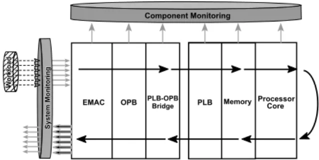
The performance evaluation done using the data collected during simulation can be distin-guished into either a component level evaluation or a system evaluation. These are illustrated in Fig. 4 (note that this shows the organization of the framework; the models of the diﬀerent

architec-tural components might vary in their level of ab-straction and details). The component evaluation is based on the data collected through the data collection layer of each component model. Exam-ples of such evaluation metrics can be memory fill levels, bus rearbitration counts, and the load on the different components. System specific aspects of an architecture like the overall system throughput, or end-to-end packet delays are evaluated using system evaluation mechanisms. In contrast to the component evaluation approach, the data in this case is not gathered within a specific component but is collected using the workload traveling through the entire system.

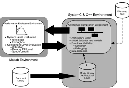
An overview of the entire simulation framework is given in Fig. 5. Based on specification docu-ments of already existing components, a set of abstract models are created and combined with component- and system-specific data collection metrics. Such models constitute, what is referred to in the figure as the ‘‘Model Library’’. The archi-tectural models from this library can be composed together and then simulated on a workload. 5.2. Component modeling

In this section we brieﬂy describe how each component of the reference network processor architecture that is evaluated in Section 6 is mod-eled in the simulation. This would enable a meaningful comparison between the results ob-tained by simulation and those obob-tained from the analytical model. The models usually available from core libraries are in the form of hard or soft cores, whereas SystemC models used in the

EMAC OPB PLB-OPB_Bridge PLB Memory Component Monitoring Processor Core S y s te m System M o n it o ri n g Monitoring W o rk lo a d W o rkload

Fig. 4. System evaluation and component evaluation of a net-work processor architecture.

(12)

simulation were created for the work done in [32]. The discussion below refers to these SystemC models.

5.2.1. Bus models

The bus models used in the reference ture are based on the CoreConnect bus architec-ture [14], designed to facilitate core based designs. CoreConnect involves three buses: The processor local bus (PLB) is for interconnecting high per-formance cores with high bandwidth and low la-tency demands, such as CPU cores, memory controllers and PCI bridges. The on-chip periph-eral bus (OPB) hosts lower data rate periphperiph-erals such as serial and parallel ports and UARTs. The PLB is fully synchronous, has decoupled address, read and write data lines and transfers on each data line are pipelined. Diﬀerent masters maybe active on the PLB address, read and write data lines and access to the PLB is granted through a central arbitration mechanism that allow masters to compete for bus ownership.

The models used for the PLB and the OPB are both cycle accurate. Both these models do not transfer any data nor consider any address, but model the signal interchanging according to the bus protocol.

There is a third bus in CoreConnect, which we do not use in our study. This is called the device

control register (DCR) bus, and is used for reading and writing low performance status and conﬁgu-ration registers.

The features of the PLB that are modeled for our study include the arbitration mechanism, the de-coupled address and read and write lines, a ﬁxed length burst protocol, and a slave enforced arbi-tration mechanism. The OPB is much less sophis-ticated compared to the PLB and most of its features are modeled. For both the buses, the arbi-tration algorithm uses a round robin strategy among the requesting masters on a given priority level, and typically there are four priority levels.

5.2.2. Ethernet core (EMAC) model

The Ethernet core or EMAC is a generic im-plementation of the Ethernet media access control (MAC) protocol, supporting both half-duplex (CSMA/CD) and full duplex operations for Ethernet, Fast Ethernet and Gigabit-Ethernet. The EMAC has two large FIFOs to buﬀer packets, and two OPB interfaces––one for providing access to its conﬁgurations and status registers, and the other is a bidirectional interface to transfer data to and from the PLB–OPB bridge.

The model of the EMAC only contains receiv-ing and transmittreceiv-ing channels, where a receive channel can be considered as an input port and a transmit channel as an output port.

Model Library Architectural

Level

Architecture Composition Environment

Architecture Editor Model Editor for new models Functional Validation

Simulation Debugging Data Collection

Monitored Data System Level Evaluation

Rx/Tx rate Throughput

Component Level Evaluation Utilization

Memory Fill Level Queue Length

ts

SystemC & C++ Environment

Matlab Environment Performance Evaluation Environment

Workload Suit

Document Library

Fig. 5. Overview of the simulation framework that is used for comparing the results obtained by the analytical method with simulation results.

(13)

The set of receiving channels constitutes the traffic input to the network processor. Each one reads packet information from a real traffic trace at a parameterizable rate. Within a receive channel there are two threads of activity. The first one reads the input packet traces, and writes each re-sulting packet into a FIFO. The second thread implements the communication protocol with the PLB–OPB bridge and transfers packets to memory as long as the FIFO is not empty. The transmit

path consists only of a transmit packet thread,

which is active as long as packets are waiting to be transferred to the appropriate port.

5.2.3. PLB–OPB bridge model

The PLB–OPB bridge is a specialized module which combines pure bridge functionality with DMA capability, and it can eﬀectively handle packet transfer overheads. An EMAC communi-cates with a PLB through the PLB–OPB bridge. Since as an OPB slave, the EMAC cannot inform the bridge of its willingness to transfer a packet, the EMAC to PLB–OPB bridge interface has sideband signals to serve this purpose. These do not form a part of the OPB bus, and nearly all signals are driven by the EMAC and sampled by the bridge.

The PLB–OPB bridge is modeled as two inde-pendent paths, receive and transmit, and both oﬀer the bridge functionality and arbitrate among ac-tive channels. Each path implements the PLB– OPB bridge to EMAC communication protocol by driving the required sideband signals and accessing buses. Bus accesses are concurrent and therefore both paths can contend for their access, especially on the OPB.

5.2.4. Memory model

The memory is accessed via the PLB and can either be on-chip or oﬀ-chip. It is modeled in a high-level way, where only parameters like average or worst case transfer latency are considered. 5.2.5. Software application and timing

A simple high-level model of software applica-tion is used. It primarily consists of the following. For each packet, the software can cause a pure delay without generating any PLB load,

repre-senting processing time in the CPU. Second, there can be a PLB load generated by the software (for example, this might consist of reading and writing packets by the CPU to and from the memory). Lastly, the timing model is based on using the PLB clock as the system time.

6. A comparative study

This section presents the main result of this paper––a comparison of the performance evalua-tion data obtained by the analytical framework presented in Sections 3 and 4 on a reference net-work processor architecture, with the results ob-tained by detailed simulations based on the models discussed in Section 5. This comparative study is based on the assumption that there is a high con-ﬁdence in the simulation results. We do not com-pare the results obtained by either the analytical method or the simulations with any real hardware implementation because of two reasons: (i) During a design phase actual hardware does not exist, and the best one can do is to validate the results ob-tained from an analytical model against those obtained using simulation, and vice versa. (ii) Simulations are widely used in practice, and as-suming that the processor model being simulated is accurate and detailed enough, the results are ex-pected to match the real hardware with high con-ﬁdence.

Our choice of the reference architecture which is the basis of the comparison is a hypothetical sys-tem-level model of a network processor which can be matched by many existing network processors (such as the family of processors described in [21]). The architectural components modeled in this study are from an existing core library [13]. Since the particular system-level model we study here is suﬃciently general, we believe that the conclusions based on the results obtained from this study would hold for many other models. This enables us to make the general claim that it is possible (and more appropriate in terms of the beneﬁts in run-ning time) to use analytical modeling frameworks during the early stages of architecture design space exploration in the context of network processors, in order to tackle the design complexity.

(14)

We evaluate the reference architecture using three different performance metrics: (i) The line speed or the end-to-end throughput that can be supported by the architecture. This is measured using the utilization of the different components of the architecture and hence also identifies the component which acts as the bottleneck. During a design space exploration, identifying the utiliza-tion of the different components goes beyond measuring the overall throughput of the system because a designer is generally interested in iden-tifying whether all the components in the archi-tecture have a moderately high utilization at the maximum supported line speed, or whether it is one single component that acts as a bottleneck. (ii) The maximum end-to-end delay that is experi-enced by packets from the different flows being processed by the architecture. (iii) The total on-chip buffer/memory requirements, or in other words, the on-chip memory fill level. The results of the analytical framework should be judged on the basis of how closely the data related to these per-formance metrics for the reference architecture match those obtained using simulation. Rather than absolute values, it is more interesting to an-alyse the behavior of the architecture (for example with increasing line speeds, or increasing packet sizes for the same line speed), and see if the same conclusions can be drawn from both evaluation techniques. The second axis for our comparisons is the time it takes to compute the evaluation data by the analytical framework, compared to the simu-lation time required to generate this data.

6.1. Reference architecture and parameters

The system-level model of a network processor that is used for this study is shown in Fig. 1. The diﬀerent actions that are executed while each packet travels through this architecture, and the order in which they are executed is given in Table 1. The model eﬀectively deals with the communi-cation subsystem of the architecture, and the software application running on the CPU core (indicated by PPC-PowerPC) is modeled as simply performing two reads from the SDRAM and one write to the SDRAM for every processed packet. The amount of data read or written (and hence the

traﬃc generated on the PLB), however, depends on the packet size and this is appropriately mod-eled.

As seen in Fig. 1, the architecture is composed of two Ethernet media access controllers (EMACs), a slow on-chip peripheral bus (the OPB), a fast processor local bus (the PLB) consisting of sepa-rate read and write lines, a PLB–OPB bridge, a SDRAM and a processor core (PPC). Each EMAC consists of one receive and one transmit channel, and is capable of reading packets at pa-rameterizable input rates.

In the simulation, the entire path of a packet through the modeled architecture can be described as follows. First a receive channel of an EMAC reads a packet from a file containing the packet traces (only packet lengths are used, and all packets arrive back-to-back with a fixed inter-frame gap; this is described in further details later), and allocates a packet record which contains the packet length and the source EMAC identifica-tion. This packet record models the packet inside the processor architecture and generates a load equivalent to the size of the packet. The channel then requests service to the PLB–OPB bridge via a sideband signal, which is served following a bridge internal arbitration procedure. The PLB–OPB

Table 1

Sequence of actions for every processed packet in the archi-tecture model shown in Fig. 1

Step Action

1 Sideband signal from EMAC to bridge (indicating that a new packet has arrived)

2 Bridge gets a ‘‘buﬀer descriptor’’ (BD) from the SDRAM

3 Packet is sent from EMAC to bridge over the OPB 4 Packet is sent from bridge to SDRAM over the

PLB write bus

5 Sideband signal from Bridge to PPC (indicating that the new packet has been stored)

6 CPU get buﬀer descriptor over the PLB read bus 7 CPU gets packet header over the PLB read bus 8 CPU processes header, and stores it back to

SDRAM over the PLB write bus

9 Sideband signal from bridge to CPU (indicating that the packet can be sent out)

10 Bridge gets buﬀer descriptor over the PLB read bus 11 Bridge gets packet over the PLB read bus 12 Packet sent out to speciﬁed a EMAC over the OPB

(15)

bridge fetches a buffer descriptor for the packet (which is a data structure containing a memory address in the SDRAM, where the received packet is to be stored). This fetching operation involves the SDRAM and generates traffic on the PLB read bus, equal to the size of the buffer descriptor. Following this, the received packet is stored in the SDRAM at the location specified by the buffer descriptor. This involves the packet traversing through the OPB to the PLB–OPB bridge, and then through the PLB write bus to the SDRAM. This generates a load equal to the size of the packet, on both the buses. Since data on the PLB is sent in bursts, the PLB–OPB bridge schedules a PLB transfer only when sufficient data is gathered. As the EMAC channel is served over and over again, the packet is written part by part into the SDRAM. After the packet transfer is complete, the bridge informs the EMAC receive channel via a sideband signal, and also notifies the application software running on the processor core (again by a sideband signal) that the packet is now available in the memory. It is then processed by the software as soon as the processor becomes available. This processing involves a buffer descriptor transfer from the SDRAM to the processor core via the PLB read bus, followed by a packet header transfer, again from the SDRAM to the proces-sor core via the PLB read bus. The packet header is then processed in the processor core (for exam-ple, implementing some lookup operation) and written back into the SDRAM over the PLB write bus.

After the completion of this processing, the software notifies the bridge (via a sideband signal) that the packet is now processed and is ready to be sent out through the chosen transmit channel of the EMAC. As in the receive path of the packet, the bridge gets the buffer descriptor of the packet from the SDRAM via the PLB read bus, and then the packet traverses over the PLB read bus and the OPB to an EMAC transmit channel. After the completion of the packet transfer, the EMAC notifies the bridge via a sideband signal, which then reads certain status information and releases the buffer descriptors.

This entire process happens concurrently for two packet ﬂows entering through the two

EMACs of the architecture. All the components involved also work concurrently and the two buses (the PLB and the OPB) use FCFS as a bus arbi-tration policy. The main complexity in the analysis of this system is due to concurrent operation of the diﬀerent components. Hence it is non-trivial to evaluate how the system behaves with increasing line speeds, variations in packet sizes, and what is the maximum line speed that it can support with-out packet dropping.

6.1.1. Parameters

As already mentioned, the EMAC can read packets at diﬀerent input line speeds. The line speeds used for the evaluation range from 100 to 400 Mbps, the former representing a nominal load situation and the later a loaded situation.

The OPB modeled has a width of 32 bits and a frequency of 66.5 MHz. The read and the write data paths of the PLB are of 128 bits and operate at 133 MHz. The size of a PLB burst is limited to a maximum of 64 bytes. Therefore, the PLB–OPB bridge gathers up to 64 bytes (which is only one OPB burst transfer) before scheduling the PLB transfer. There are two different kinds of buffer descriptors, small and large ones. The small buffer descriptors refer to memory locations/buffers with 64 bytes of size, while the large ones refer to buffers with a size of 1472 bytes. As a consequence, 64 byte packets require only one small buffer de-scriptor and packets larger than 64 bytes require

an additional large buﬀer descriptor. Both small

and large buffer descriptors are of size 64 bytes each. Therefore, the traffic generated by a packet on any of the buses depends not only on its own size, but also on the buffer descriptors associated with it. All packets and the buffer descriptors re-side in the SDRAM described above.

6.2. Evaluation method and comparisons

The reference architecture described above is evaluated using simulation and the analytical framework, using two diﬀerent workload types–– synthetic traces with same-sized packets, and real traces from NLANR [18]. For the synthetic traces, packet sizes of 64, 128, 512, 1024, 1280 and 1500 bytes are used. The real traces are used only to

(16)

exploit the impact of real world packet size dis-tributions on the system performance. They are time compressed and adjusted and only the packet sizes are retained. Therefore, in both cases packets arrive back-to-back (to exert the maximum stress on the architecture) with an interframe gap equal to 20 bytes.

The overall scheme for comparing the results obtained using the analytical framework with those obtained from simulation is shown in Fig. 6. The diﬀerent components of the architecture are modeled in either SystemC in the simulation based evaluation, or analytically using the model pre-sented in Section 3. To compute the required pa-rameters of an analytical component model (such as the transfer time of a single packet over an unloaded bus), either simulation results or data sheets of the component are used. The component models are then composed together (using the methods described in Section 4 in the case of the analytical framework, and using standard SystemC composition techniques in the case of simulation) to obtain a system model of the ar-chitecture.

Recall that the analytical model considered here does not use real packet traces, but instead uses arrival curves modeling the traces in terms of their maximum packet size, burstiness, and long-term arrival rate. These parameters were extracted from the traces as shown in Fig. 7 and fed into the model for evaluation. For the upper arrival curve, the maximum number of bytes that can arrive (at the network processor) at any time instant is given by the largest sized packet, the short-term burst rate is given by the maximum number of largest

sized packets that can be seen occurring back-to-back in the trace, and the long-term arrival rate is given by the total length (in bytes) of the trace divided by the time interval over which all the packets in this trace arrive.

Similarly, for the lower arrival curve, the max-imum time interval over which no traﬃc can arrive is equal to the interframe gap in the trace (equal to 20 bytes), the bound on the minimum number of bytes that can arrive over a time interval is given by the maximum number of minimum sized pack-ets occurring back-to-back in the trace, and the long-term arrival rate is equal to that in the upper arrival curve.

Given any packet trace, arrival curves such as those shown in Fig. 7 can be derived from the trace and they capture the traﬃc arrival pattern given by the trace. Note that here we restrict each arrival curve to be made up of a combination of three line segments in order to simplify the computations involving these curves. However, in general they can be arbitrarily complex to capture the exact details of a trace (albeit, at the cost of increasing the computational complexity). As mentioned in Section 4 the analytical model composes the

dif-ferent component models, resulting in ascheduling

network. For the architecture we study here (Fig. 1), such a scheduling network is given in Fig. 2. 6.3. Evaluation results

Table 2 gives the utilization values of the three buses (the OPB, and the PLB read and write bus) when the model is fed with synthetic traces

con-Fig. 6. The overall scheme for comparing the results from the analytical framework with those obtained by simulation.

Trace: cycles packet Arrival Curve: cycles Bytes

max. packet size only largest packets

average rate

only smallest packets longest gap

Fig. 7. Obtaining arrival curves from packet traces in the an-alytical framework.

(17)

sisting of fixed sized packets. Here, six different packet sizes have been used, from 64 to 1500 bytes. For each packet trace and bus combination, the table compares the results obtained from the ana-lytical method with those resulting out of simula-tion for different line speeds. To give an impression of how the utilization of the different buses increase with the line speed for the same packet size, in Fig. 8 we plot the utilization values for the trace con-taining 512 byte sized packets. As can be seen from Table 2, the results for the other traces are very similar, and hence we do not plot them.

There are two things to be noted from these values. First, with increasing line speeds the utili-zation of the diﬀerent buses also increase, and as expected, this increase is proportional to the in-crease in the line speed. Second, the results from

0 10 20 30 40 50 60 70 80 90 100Mbps 150Mbps 200Mbps 250Mbps 300Mbps 350Mbps 400Mbps Linespeed Utilization [%] Simulation Analytical Method OPB PLB read PLB write

Fig. 8. Utilization values for diﬀerent line speeds for the trace containing 512 byte packets. In this bar graph, for each line speed, the ﬁrst bar indicates the utilization of the OPB, the sec-ond bar shows the utilization of the PLB read bus and the third bar corresponds to the PLB write bus. For each bus, the white bar gives the result computed by the analytical method, and the black bar gives the result obtained from simulation.

Table 2

The utilization values of the OPB, and the PLB read and write buses, when the model is fed with six diﬀerent synthetic traces consisting of ﬁxed size packets (ranging from 64 to 1500 bytes)

OPB PLB read PLB write AnM Sim AnM Sim AnM Sim

Packet size 64 bytes

100 Mbps 18 18 14 13 6 5 150 Mbps 27 28 20 19 9 8 200 Mbps 36 37 27 25 12 10 250 Mbps 45 46 34 31 15 13 300 Mbps 54 55 41 37 17 15 350 Mbps 63 65 48 40 20 17 400 Mbps 72 76 55 47 23 20

100 Mbps 20 20 6 6 3 2 150 Mbps 30 30 9 9 4 4 200 Mbps 40 40 12 12 6 5 250 Mbps 50 50 14 15 7 6 300 Mbps 61 60 17 18 9 7 Table 2 (continued)

OPB PLB read PLB write AnM Sim AnM Sim AnM Sim

350 Mbps 72 70 20 21 10 8

400 Mbps 83 80 23 24 12 9

For each trace and for each bus, the ﬁrst column (marked as AnM-analytical method) gives the results obtained using the analytical model, and the second column (marked as Sim) gives the results obtained by simulation.

(18)

the analytical method and the simulation match very well for the utilization values. In Fig. 8, for each line speed there are three bars, each corre-sponding to the OPB, the PLB read and the PLB write bus. It may be noted from the ﬁgure that the maximum line speed that this architecture can sustain is in the range of 400 Mbps and the OPB acts as a bottleneck (as most of the traﬃc is gen-erated on it).

In Fig. 9 we show the utilization values of the PLB read bus for fixed line speeds, as the packet size is increased. For a fixed line speed, as the packet size is increased, the component of the utilization that comes from the packet traversal increases, since there is less total interframe gap in the whole trace (assuming that the trace size in bytes remains the same). This is because the number of packets in the trace decrease. However, because of this, the number of buffer descriptor and packet header traversals also decrease and therefore the component of the bus utilization that comes from these also decrease. These effects can be seen in Fig. 9. As the packet size is doubled from 64 to 128 bytes, the first component men-tioned above plays a dominating role and hence the utilization slightly increases. Thereafter, the effect of the second component dominates and the utilization falls, and then remains almost constant since there is no significant change in the number of packets as the packet size is increased from 1024 to 1280 bytes and then from 1280 to 1500 bytes. The same results for the OPB is shown in Fig. 10. However, in this case the utilization increases with

increasing packet size because these are no packet header or buﬀer descriptor transfers over this bus. It is to be noted that the match between the analytical results and the simulation is always close enough to deduce the above conclusions from the analytical results itself (with signiﬁcant savings in evaluation time).

For the ﬁxed size packet traces, we do not consider the end-to-end packet latencies and the memory ﬁll levels, since for all low load situations they remain constant and do not depend on the input line speed.

We next consider the results generated by real traces obtained from NLANR [18]. We use three different traces––FL (traces from a number of Florida universities), SDC (traces collected from the San Diego Supercomputer Center) and TAU (traces from the Tel Aviv University). Each trace is made up of traffic patterns for two different lines and these are fed into the two EMACs in our ar-chitecture. The main motivation behind using these traces is to see the effect of real-life packet size distributions on the architecture. The line speeds used for all the traces vary from 100 to 400 Mbps as before.

Figs. 11–13 show the variation in the utilization of the three different buses for the different line speeds. It maybe noted that, as before, there is a close match between the results from the simula-tion and the analytical framework. Secondly, the architecture behaves almost identically for the different traces. 0 5 10 15 20 25 30 35 40 64 128 512 1024 1280 1500 Packet Size [Bytes]

Utilization [%] 250 Mbps 200 Mbps 150 Mbps 100 Mbps Simulation Method Analytical

Fig. 9. The variation of the PLB read bus utilization with in-creasing packet size for four diﬀerent line speeds.

0 10 20 30 40 50 60 64 128 512 1024 1280 1500 Packet Size [Bytes]

Utilization [%] 100 Mbps Simulation Analytical Method 250 Mbps 200 Mbps 150 Mbps

Fig. 10. The variation of the OPB utilization with increasing packet size for four diﬀerent line speeds.

(19)

Recall that the bus arbitration mechanism used in our reference architecture is always FCFS. Unfortunately, for FCFS there do not yet exist tight bounds for delay and backlog in the analyt-ical framework that we consider here (there do exist tight bounds for static priority, round-robin, time division multiplexing, etc.). To get around this problem, we use fixed priority based arbitra-tion mechanisms in the analytical model and compare them with FCFS used in the simulation. Towards this, one of the packet flows (recall that each trace is made up of two flows) in a trace is assigned a higher priority over the other in all the buses. For computing the end-to-end packet la-tency, the maximum delay experienced by the lower priority flow now gives an upper bound on the maximum delay experienced by any packet when FCFS is used. Similarly, we use the maxi-mum delay experienced by the higher priority flow as a lower bound on the maximum delay experi-enced by any packet in the case of FCFS. These results are shown in Figs. 14–16 for the three dif-ferent traces. Note that in all the three cases, the delay values obtained through simulation lie in between the delay values (obtained from the ana-lytical method) for the high and the low priority flows. These results indicate that the architecture is sufficiently provisioned for one flow, even for high line speeds, since the maximum delays experienced 0 10 20 30 40 50 60 70 80 90 100Mbps 150Mbps 200Mbps 250Mbps 300Mbps 350Mbps 400Mbps Linespeed Utilization [%] Simulation Analytical Method OPB PLB read PLB write

Fig. 11. The utilization of the OPB and the PLB read and write buses under diﬀerent line speeds for the FL packet trace.

0 10 20 30 40 50 60 70 80 90 100Mbps 150Mbps 200Mbps 250Mbps 300Mbps 350Mbps 400Mbps Linespeed Utilization [%] Simulation Analytical Method OPB PLB write PLB read

Fig. 12. The utilization of the OPB and the PLB read and write buses under diﬀerent line speeds for the SDC packet trace.

0 10 20 30 40 50 60 70 80 90 100Mbps 150Mbps 200Mbps 250Mbps 300Mbps 350Mbps 400Mbps Linespeed Utilization [%] Simulation Method Analytical OPB PLB write PLB read

Fig. 13. The utilization of the OPB and the PLB read and write buses under diﬀerent line speeds for the TAU packet trace.

0 5000 10000 15000 20000 25000 100Mbps 150Mbps 200Mbps 250Mbps 300Mbps 350Mbps 400Mbps Linespeed Delay [PLB Cycles] Analytical Method Upper Bound Analytical Method Lower Bound Simulation

Fig. 14. The maximum end-to-end delays experienced by packets of the FL trace under different line speeds. For the two flows that make up this trace, the analytical results show the delay experienced by the higher and the lower priority flows when using priority based arbitration at the buses. The simu-lation results are based on FCFS implemented at all the buses.