An Integrated Framework for Responsive Supply Chain
Management
1
Darshit Parmar
1Teresa Wu
1John Fowler
2Tom Callarman
3Vincent Hargaden
4
Eamonn Ambrose
1Philip Wolfe
1Department of Industrial Engineering Arizona State University, PO Box 875906
Tempe, Arizona 85287-5906, USA 2
China Europe International Business School 699 Hongfeng Road, Pudong Shanghai, P. R. China 201206
3
UCD School of Business University College Dublin Belfield, Dublin 4, Ireland 4
National Institute of Technology Management University College Dublin
Belfield, Dublin 4 ABSTRACT
In today’s highly dynamic, globalized and competitive environment, companies are under pressure to improve their supply chain strategies in order to be more responsive to customer demands. Indeed the geographically distributed nature as well as the differing objectives across these dispersed entities of a supply chain can often lead to difficulties in making a supply chain responsive. Additionally, irregularities and disruptions occurring at any point in the system make responsive supply chain management even more challenging. These disruptions, often occurring without warning due to the dynamic nature of a supply chain, can lead to poor performance of the supply chain. A key component in responsive supply chain management is the ability to effectively “sense and response” in order to maximize responsiveness and flexibility and avoid system disruptions. Recent advances in communication can facilitate the sensing and data collection. However, the huge amount of data generated can impede effective response, particularly, when some data may be incomplete or have errors. Inaccurate estimate or sensing of the system state can lead to incorrect decisions, with consequent adverse effects on supply chain performance. To address this issue, this research proposes a Kalman filter based approach for exception detection. Some preliminary work, specifically, with a focus on the manufacturing portion of the IBM supply chain for server fulfillment is presented in this paper. The results show system estimation can be improved by using a Kalman filter.
1.INTRODUCTION
Supply Chain Management (SCM) emphasizes the integration of activities and information flows while focusing on increasing value for the customer. The diversity of participants in terms of size, technological capabilities, cultural differences, efficiencies etc. makes SCM a difficult task. Two additional difficulties are: (1) the presence of uncertainty in such aspects such as customer requirements (demand), capacity, transportation time, manufacturing time, costs, quality, due dates, priorities, etc. and (2) the reality of missing information, ambiguous information, and the bullwhip effect [1]. Recent developments in communication technologies and standards make improved data sharing feasible and assist the decisions on managing and controlling the operations. However, in practice, the data collected may be incomplete, inaccurate and inconsistent. Based on such data, the provision of accurate estimates of the state of a supply chain for decision making is questionable. Therefore, there is a need to improve system
estimation when incomplete data and errors in the data are present. The intent of this paper is to take an initial step forward in this direction.
Considering an IBM server fulfilment supply chain, each manufacturing facility faces a big challenge to meet the quota at the end of each quarter. The cost of an unfulfilled order can run into millions and thus it is extremely important to sense any potential exceptions that might occur. Better sensing of the manufacturing states and better estimation of the processing states can help to manage the supply chain responsively and effectively. However, manufacturing data collection is prone to measurement errors. This is largely due to the fact that where automated systems don’t exist, the operators wait for a group of jobs to complete, and then scan them into the system. In addition, such errors are very common during shift changeovers. While the completed jobs wait to be handled, the operators of the first shift pass on information to the second shift operators. This induces bias in the estimation of the cycle time and can throw off any prediction mechanisms which might be in place to estimate the final job completion.
Kalman filters have traditionally been used for stochastic estimation and control. They have been used to obtain better state estimations. In this work, a Kalman filter approach is used to take into account the measurement errors and to obtain a better state estimation, namely the estimated start and end processing times of the jobs. A better state estimation ultimately leads to better estimation of the final job completion. In addition to obtaining a better estimation of the final job completion, a new approach is proposed to calibrate the path that a job is expected to take over time. In other words, as and when more information is obtained, the expected travel path of the jobs changes over time and these changes are incorporated in real time to obtain a better idea of whether a job is on course for timely completion or not. This approach is used to sense any potential exceptions that might occur. The format of the paper is as follows. First, the background of Kalman filters is reviewed followed by the applications of Kalman filters. Then, the basis of the proposed approach is described. Finally, an example is presented followed by conclusions and ideas for future research.
2. BASICS OF KALMAN FILTERS
The Kalman filter provides an efficient computational (recursive) means to estimate the state of a process [2]. Kalman [3, 4] formulates the Wiener problem, a filter problem for communication and control from the “state” point of view and the resulting Kalman filter is recursive solution to the discrete-data linear filtering problem. A Kalman filter is a set of mathematical equations that supports estimations of past, present, and even future states. The power comes from the fact that it can do these estimations even when the precise nature of the modeled system is unknown [2]. Figure 1 shows the general procedure of Kalman filter.
Figure 1: Typical Kalman filter Application (Adopted from [5])
Mathematically, a Kalman filter is a set of recursive equations used to estimate the state x ∈ Rn of a discrete-time controlled process such as manufacturing process that is governed by the transition equation and measurement equation.
Transition Equation: xk = G*xk-1 + εk-1, x∈R n Measurement Equation: zk = H* xk + ηk, z∈R m
Where Gnxn is the system state matrix that relates the state at the previous time step k-1 to the present step k, Hmxn relates the system states to the measurements. The random variables εk and ηk represent the process and measurement noise respectively. They are assumed to be white noise with normal distributions: p (εk) ∼ N (0, Qk) and p (ηk) ∼ N (0, Rk). The equations for the Kalman filter fall into two groups: time based equations (Equation 1 and 2), applied to obtain the current system state, and measurement based equations (Equation 3-5), used to adjust the system state from the measurements.
where Kk is the Kalman gain, Pk is the error covariance, is the estimation of x k before the measurement, and is the estimation of x k given measurement zk. The Kalman filter assembles the two groups of equations to give the best estimate of the system state. The system of measurement and transition equations can be combined into an iterative process to determine the state of the system x.
The Kalman filter has been applied in a variety of applications including Inertial Navigation and Guidance [6], Global Positioning Systems [7], Target Tracking [8], Finance [9, 10], etc. In the domain of supply chain, Aviv [11] proposes an adaptive inventory replenishment policy that utilizes the Kalman filtering technique. Wu and O’Grady [12] develop an integrated approach that uses Kalman filtering and Petri Net model to obtain a better state estimation of the supply chain system. Vensim [http://www.vensim.com/], an optimizer tool provided by Ventana Systems, uses Kalman filtering to track the actual inventory and claim that Kalman filtering tracks the inventory much better than either simple simulation alone or the measured inventory alone. This research aims to explore the application of Kalman filter to an IBM manufacturing process in the context of a “sense and response” supply chain.
3. DESCRIPTION OF THE APPROACH
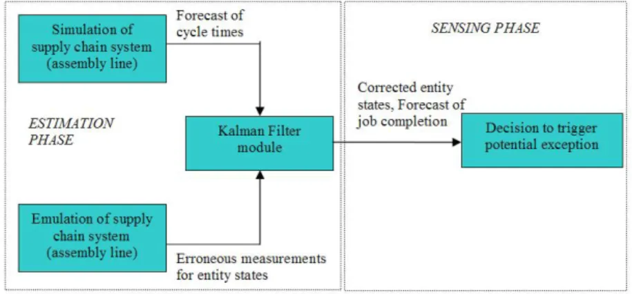
As shown in Figure 2, the proposed approach can be divided into two phases: the estimation phase and the sensing phase. In the estimation phase, an estimate of when the job will complete the final process is obtained, based on what has been happening. Predicted finishing time is obtained by running a simulation module. When a job is in a process, an emulation module provides real progress. The Kalman filter module will calibrate the results and provide a more realistic estimate. Given an improved estimate, a sensing phase will determine whether the job will come out as scheduled.
Figure 2. Proposed Framework
1 1 ˆ ˆ (1) k k T k k k x Gx P G P G Q − − − − = = + 1 (2) ( ) (3) ˆ ( ˆ ) T T k k k k k k k k k K P H HP H R x x K z H x − − − − − = + = + − (4) ( ) (5) k k k P = −I K H P− − k xˆ k xˆ
3.1.NOMENCLATURE
Li Time when entity starts or completes aprocess. For example, L1 refers to the start of the first process, L2 refers to the end of the first process, L3 refers to the start of the second process, and so on.
EAT Entity arrival time
TB(EAT→L1) Estimate of time between entity arrival and start time of the first process
TB(Li→Li+1) Estimate of time between the instant when entity is at the starting of process and the end of the process. This accounts for the queue time between the end and beginning of a process and the processing time at a process.
(
L L12)
TB i→ Estimate of time between the start of one process to the end of the overall process
( )
L
iEst
Estimated time for entity to be at the start or the end of the process( )
L
iMsd
Measured time for entity to be at the start or the end of the process( )
L
iCor
Corrected time for entity to be at the start or the end of the process( )
L
iK
Kalman correction(
Est
L
i)
2ˆ
σ
Estimate of variance in estimated time ofL
i(
Msd
L
i)
2ˆ
σ
Estimate of variance in measured ofL
i (assumed to be 36)(
Cor
L
i)
2ˆ
σ
Estimate of variance in corrected time ofL
i(
)
(
1)
2
ˆ
T
B
E
AT→
L
σ
Estimate of variance in estimated time between entity arrival time and the start time of the first process(
)
(
)
2 1 ˆ TB Li Liσ →+ Estimate of variance in estimated time between the instance when entity is at the start and the end of the process
(
)
(
12)
2
ˆ TB Li →L
σ Estimate of variance in estimated time between the start of one process and the end of the overall process
3.2.PROBLEM SPECIFICATION
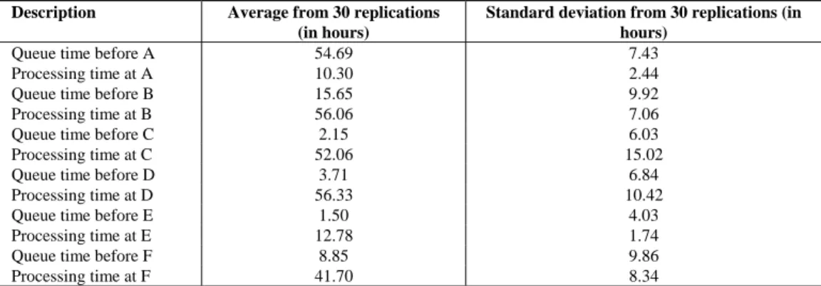
This research studies the IBM server manufacturing process, a six step serial process that is identified as shown in Figure 3. The processing time distribution for all six processes is triangular with the parameters shown in Table 1.
Figure 3: Six step serial process
Table 1: Assumed parameters of triangular distribution for processing time at each process
Process Low (in hours) Mode (in hours) High (in hours)
A 6 8 17 B 30 60 75 C 18 35 92 D 30 60 80 E 8 13 17 F 25 45 60
The time between arrivals of entities (or jobs) is assumed to be exponentially distributed with a mean of ten hours. It is also assumed that there is a provision to take measurements (or collect information) on the start and the
end times at every process for every entity, and there are errors in these measurements and that these errors are normally distributed.
3.3. ESTIMATION PHASE
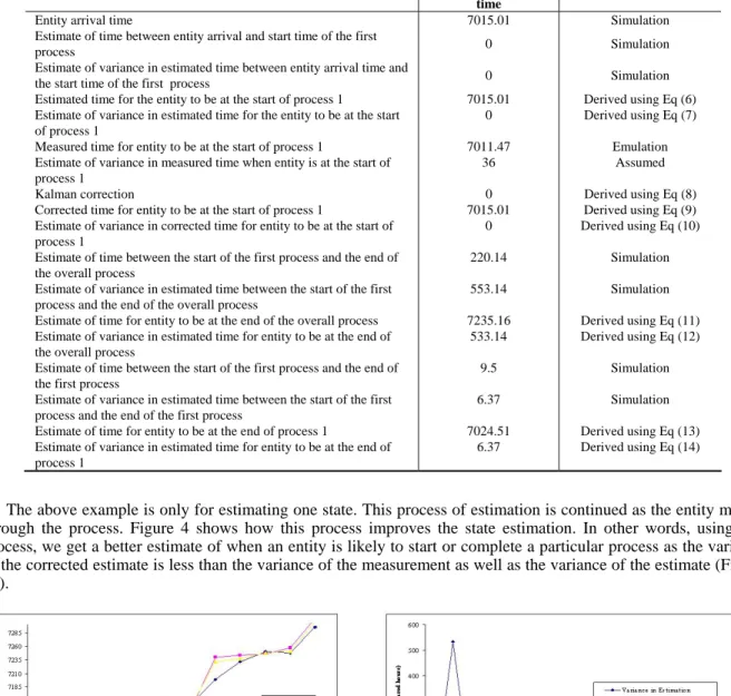
First, an estimate of when an entity will pass through every process is obtained. This estimate is obtained using simulation. The entire process is simulated for 30 replications. For each replication, the arrival time of the entity to the system, is kept the same. An estimate of the queue times for all entities and an estimate of the processing times for all entities at every process are calculated by taking the average from the 30 replications. The standard deviation in these estimates is also calculated. Table 2 gives an example of what these numbers might look like for one particular entity.
Table 2: Estimated queue times and processing times for a sample entity
Description Average from 30 replications (in hours)
Standard deviation from 30 replications (in hours)
Queue time before A 54.69 7.43
Processing time at A 10.30 2.44
Queue time before B 15.65 9.92
Processing time at B 56.06 7.06
Queue time before C 2.15 6.03
Processing time at C 52.06 15.02
Queue time before D 3.71 6.84
Processing time at D 56.33 10.42
Queue time before E 1.50 4.03
Processing time at E 12.78 1.74
Queue time before F 8.85 9.86
Processing time at F 41.70 8.34
To emulate the real world, an additional simulation is run, using the same distribution and using the same parameters for the processing times as used in the simulation with 30 replications. We call this emulation. In other words, measurements obtained from emulation are assumed to represent measurements obtained from the real world. At this point, information from two different sources is available and both these sources have variability – simulation has variance in estimation and emulation has variance in measurement. These two pieces of information are now combined using equations (6) – (14) to obtain a better estimate of the job completion. Equation (6) estimates the start time of the process at process A. Equation (7) estimates the variation in the estimate of the start time. Equation (8) calculates the Kalman correction required to account for the measurement error in the state. Equation (9) applies the Kalman correction and obtains the corrected estimates of the state. Equation (10) estimates the variance in the corrected estimate of the state. Equation (11) uses the corrected estimate for intermediate states to estimate when an entity will complete the last process (process F). Equation (12) estimates the corrected variance in the estimate of the state when an entity will complete the last process (process F). Equation (13) estimates the next entity state from the corrected current state. Equation (14) estimates the variance in the estimate of the next entity state.
( )
L
1E
TB
(
E
L
1)
Est
=
AT+
AT→
(6)(
)
(
(
)
)
(
(
1)
)
2 1 2 1 2ˆ
ˆ
ˆ
Est
L
=
σ
E
AT+
TB
E
AT→
L
=
σ
T
B
E
AT→
L
σ
(7)( )
ˆ
2(
)
/
(
ˆ
2(
)
ˆ
2(
)
)
i i i iEst
L
Est
L
Msd
L
L
K
=
σ
σ
+
σ
(8)( )
L
iEst
( )
L
iK
( )
L
i(
Msd
( )
L
iEst
( )
L
i)
Cor
=
+
*
−
(9)( )
(
Cor
L
i)
(
Est
L
i)
K
( )
L
i(
Est
L
i)
2 2 2ˆ
*
ˆ
ˆ
σ
σ
σ
=
−
(10)( )
L
12Cor
( )
L
TB
(
L
L
12)
Est
=
i+
i→
(11)( )
(
)
(
( )
)
(
(
12)
)
2 2 12 2ˆ
ˆ
ˆ
Est
L
=
σ
Cor
L
i+
σ
TB
L
i→
L
σ
(12)( )
L
i+1=
Cor
( )
L
i+
TB
(
L
i→
L
i+1)
Est
(13)( )
(
)
(
( )
)
(
(
1)
)
2 2 1 2ˆ
ˆ
ˆ
Est
L
i+=
σ
Cor
L
i+
σ
TB
L
i→
L
i+σ
(14)Note that the numbers used to show the start and the completion times of an entity at a process are in terms of the simulation clock time. Also, the estimates of time are in hours. Thus, variance is in terms of squared hours.
[Example]
Table 3 gives an example of how equations (6) – (14) can be applied to estimate the states of the entity as it moves through the process.
Table 3: Example showing state estimation for one sample entity Parameter Description Simulation clock
time
Source
Entity arrival time 7015.01 Simulation
Estimate of time between entity arrival and start time of the first
process 0 Simulation
Estimate of variance in estimated time between entity arrival time and
the start time of the first process 0 Simulation
Estimated time for the entity to be at the start of process 1 7015.01 Derived using Eq (6) Estimate of variance in estimated time for the entity to be at the start
of process 1
0 Derived using Eq (7) Measured time for entity to be at the start of process 1 7011.47 Emulation Estimate of variance in measured time when entity is at the start of
process 1
36 Assumed
Kalman correction 0 Derived using Eq (8)
Corrected time for entity to be at the start of process 1 7015.01 Derived using Eq (9) Estimate of variance in corrected time for entity to be at the start of
process 1
0 Derived using Eq (10) Estimate of time between the start of the first process and the end of
the overall process
220.14 Simulation Estimate of variance in estimated time between the start of the first
process and the end of the overall process
553.14 Simulation Estimate of time for entity to be at the end of the overall process 7235.16 Derived using Eq (11)
Estimate of variance in estimated time for entity to be at the end of the overall process
533.14 Derived using Eq (12) Estimate of time between the start of the first process and the end of
the first process
9.5 Simulation Estimate of variance in estimated time between the start of the first
process and the end of the first process
6.37 Simulation Estimate of time for entity to be at the end of process 1 7024.51 Derived using Eq (13)
Estimate of variance in estimated time for entity to be at the end of process 1
6.37 Derived using Eq (14)
The above example is only for estimating one state. This process of estimation is continued as the entity moved through the process. Figure 4 shows how this process improves the state estimation. In other words, using this process, we get a better estimate of when an entity is likely to start or complete a particular process as the variance of the corrected estimate is less than the variance of the measurement as well as the variance of the estimate (Figure 4b).
(a) (b)
3.3. SENSING PHASE
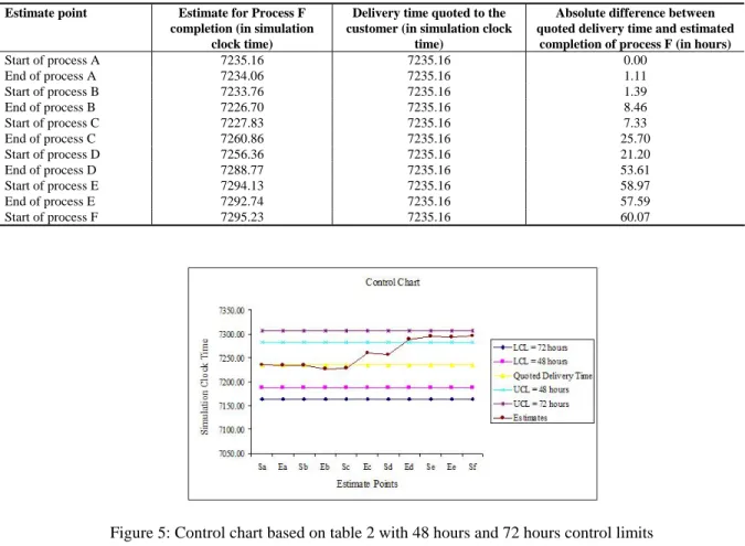
It is assumed that there is a method in place for quoting the delivery date to the customer. For our purposes, it is assumed that the delivery date is determined based on the results from 30 replications of the simulation. Also, the delivery date is in terms of the simulation clock time. The steps for sensing exceptions are explained below with an example. Suppose that we are interested in determining how entity number 516 is doing. The estimated completion time from 30 replications of simulation for this entity is 7235.157 (in terms of simulation clock time). In other words, this entity is expected to complete process F at 7235.157. Suppose that this is the time quoted to the customer. Now, when the entity is actually going through each of the six processes, we apply the Kalman filter corrections and re-estimate its completion time. These estimates, which are changed in real time, can be used to compare with the completion time quoted to the customer. And depending on the amount of tolerable risk, a control chart can be plotted. For example, suppose that we want to know whether the entity is likely to take more than 2 days than the quoted time to the customer. Table 4 below summarizes the results showing the difference between the delivery time quoted to the customer and the estimated process F completion from different estimate points, for one entity.
Table 4: Example showing the calculation of difference between the delivery time quoted to the customer and the estimated process F completion from different estimate points for one entity
Estimate point Estimate for Process F completion (in simulation
clock time)
Delivery time quoted to the customer (in simulation clock
time)
Absolute difference between quoted delivery time and estimated
completion of process F (in hours)
Start of process A 7235.16 7235.16 0.00 End of process A 7234.06 7235.16 1.11 Start of process B 7233.76 7235.16 1.39 End of process B 7226.70 7235.16 8.46 Start of process C 7227.83 7235.16 7.33 End of process C 7260.86 7235.16 25.70 Start of process D 7256.36 7235.16 21.20 End of process D 7288.77 7235.16 53.61 Start of process E 7294.13 7235.16 58.97 End of process E 7292.74 7235.16 57.59 Start of process F 7295.23 7235.16 60.07
Figure 5: Control chart based on table 2 with 48 hours and 72 hours control limits
To determine whether this method sensed accurately or not, we used the final corrected completion time for end of process F. A difference between the quoted delivery time to the customer and the corrected completion time for end of process F was computed. The threshold is set as 48 hours, that is, if the control chart signaled when the difference exceeded 48 hours, it was considered as correct classification. On the other hand, if this difference was less than 48 hours, and if the control chart signaled, it was considered as an inaccurate classification. In this preliminary research, we set the threshold based on experience. More experiments need to be done to tune this parameter to account for the tolerable risk. Same calculations were performed for all entities and the results are summarized in Table 5.
Table 5: Results for all entities
Description Number
Total number of entities 1000
Total signals 33
Correct signals 15
False signals 14
Missed signals 4
As shown in Table 5, there were 1000 total entities to which the above described approach was applied. There were signals for 29 entities. No signal was later than the end of process E. There were 15 correct signals and 14 incorrect signals. Out of the 14 incorrect signals, there were 6 entities which differed from the quoted delivery date to the customer by more than 40 hours. They were incorrect because the control chart signaled that these entities would take more than 48 hours than the quoted delivery date. We call these 6 signals as close false signals. In addition, there were 8 other false signals meaning that the control chart indicated that these entities would take more than 48 hours, whereas in reality, these entities did not exceed 48 hours. Also, there were 4 missed signals. These were the entities which took more than 48 hours, but the control chart did not signal. The overall accuracy using this approach to sense exceptions is (1000 – 18) / 1000 = 98.2%.
5.SUMMARY
One management strategy for a responsive supply chain is “sense and response” which requires continuously monitoring business process, detecting existing or anticipated business issues, resolving these issues as early as possible. This paper proposes an integrated framework for “sensing”, utilizing simulation techniques and a Kalman filter. In particular, an IBM server fulfillment supply chain is studied. To validate the proposed framework, we concentrate on the server manufacturing process. The results indicate that using a Kalman filter can help in getting a more realistic estimate of when an entity is likely to come out of the factory. The improved estimates are then used to sense whether an entity is on course to meet customer delivery expectations. In the future, it is intended to repeat the estimation and sensing phases at other IBM server manufacturing sites. We will then explore the application of the proposed framework to a fully fledged supply network. In addition, more scenarios such as different types of exceptions in the sensing phase need to be explored. Finally, we will develop a response model when exceptions are sensed.
REFERENCES
[1] J., Blackhurst, J., T., Wu and P., O’Grady, “Network-based approach to modeling uncertainty in a supply chain”, International Journal of Production Research, 15, 42, 8, 2004, pp.1639-1658.
[2] G. Welch and G. Bishop: “An introduction to the Kalman filter”, Technical Report No. TR 95-041, Department of Computer Science, University of North Carolina, 1995.
[3] R.E. Kalman, and R.S. Bucy., "New Results in Linear Filtering and Prediction Theory", Transactions of the ASME series D: Journal of Basic Engineering, 83 (3): 95 - 108, 1961.
[4] R.E. Kalman, "A New Approach to Linear Filtering and Prediction Problems", Transactions of the ASME series D: Journal of Basic Engineering, 82 (1): 35 - 45, 1960.
[5] P. S. Maybeck: “Stochastic Models, Estimation, and Control”, Vol 1, Academic Press, Inc., New York, 1979. [6] P. Zarrchan., "Tactical and Strategic Missile Guidance", AIAA, Inc., Washington, DC, 1994.
[7] R.P. Denaro and P.V.W. Loomis., "GPS Navigation Processing and Kalman filtering", AGARD, NO. 161, pp. 11.1-11.9, 1989.
[8] C. K. Chui and G. Chen, Kalman filtering with Real-Time Applications, Springer-Verlag, New York, 1987. [9] C. Wells, "The Kalman filter in Finance", Kluwer Academic Publishers, Dordrecht, 1995.
[10]P.J. Bolland and J.T. Connor, "A Constrained Neural Network Kalman filter for Price Estimation in High Frequency Financial Data", International Journal of Neural Systems, Vol. 8., No. 4, August, 1997.
[11] Y. Aviv: “A Time Series Framework for Supply Chain Inventory Management”, Operations Research, Vol. 51, No. 2, pp. 210-227, 2003.
[12] T. Wu and P. O’Grady: “A Methodology for Improving the Design of a Supply Chain”, International Journal of Computer Integrated Manufacturing, Vol. 17, No. 4, pp. 281-293, 2004.
![Figure 1: Typical Kalman filter Application (Adopted from [5])](https://thumb-us.123doks.com/thumbv2/123dok_us/425042.2548801/2.918.299.665.691.947/figure-typical-kalman-filter-application-adopted.webp)