Parametric Programming in Control Theory

(1)

PARAMETRIC

P

ROGRAMMING IN

CONTROL

THEORY

THESIS BY JØRGENSPJØTVOLD

Submitted in partial fulfillment of the requirements for the degree of philosophiae doctor, control engineering

DEPARTMENT OFENGINEERINGCYBERNETICS NORWEGIAN UNIVERSITY OF SCIENCE AND TECHNOLOGY

N-7491 TRONDHEIM, NORWAY MAY 2008

(2)

Norwegian University of Science and Technology

Faculty of Information Technology, Mathematics and Electrical Engineering Department of Engineering Cybernetics

N-7491 Trondheim Norway Ph. D. Thesis: 2008:94 ITK Report: 2008-5-W ISBN: 978-82-471-7880-5 (Electronic) ISBN: 978-82-471-7877-5 (Printed) ISSN: 1503-8181

(3)

Summary

The main contributions in this thesis are advances in parametric programming. The thesis is divided into three parts; theoretical advances, application areas and con-strained control allocation. The first part deals with continuity properties and the structure of solutions to convex parametric quadratic and linear programs. The sec-ond part focuses on applications of parametric quadratic and linear programming in control theory. The third part deals with control allocation. This thesis is mainly a collection of articles where each article has been slightly modified. Note that several definitions differ from paper to paper (chapter to chapter).

Chapter 2 presents a novel method for obtaining a unique polyhedral represen-tation of a continuous selection for convex parametric quadratic programs (which includes parametric linear programs). The main contribution is to utilize a two-level optimization method to obtain theminimum norm solution.

Chapter 3 introduces the so-calledfacet-to-facet propertyfor parametric pro-grams. It is pointed out that the correctness of several existing algorithms depend upon this property being satisfied. It is relatively simple to set up examples for convex parametric quadratic programs where the facet-to-facet property fails, how-ever, forstrictly convexquadratic programs it is rarely seen. It is exemplified that the facet-to-facet property does not hold for strictly convex parametric quadratic programs. A new exploration strategy is proposed to remedy this problem.

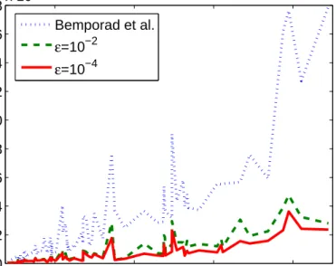
In Chapter 4 a method for obtaining explicit solutions toinf–supcontrol of constrained discrete–time discontinuous piecewise affine system subject to state-and input-dependent disturbances is presented. For this problem a solution is not guaranteed to exist. When a solution does not exist, a sub-optimal solution is obtained and a bound on the sub-optimality is given. The method allows for the degree of sub-optimality to be specifieda priori.

Chapter 5 presents a method that utilizes the dynamics of a discrete-time sys-tem to reduce the computational effort needed to evaluate the piecewise affine con-trol law. The explicit concon-trol law and structure of the dynamic system makes it possible to map a polyhedral set one step forward in time. We demonstrate how thisone-step forward reach set can be utilized to speed up the evaluation of the control law at the next sample instant.

Chapter 6 presents a case study and experimental results for constrained control allocation for a scale model of athruster-controlled floating platform. An explicit solution to a convexified problem is computed and experimental results document

(4)

ii

the performance.

In Chapter 7 a decomposition strategy for constrained linear control allocation problems is presented. The problem is divided into a master and a set of sub-problems for the purpose of obtaining a feasible, but possibly sub-optimal, solu-tion. The decomposition strategy provides flexibility for the designer, for instance a mix of online optimization and explicit solutions can be employed. We also il-lustrate how the decomposition strategy can be utilized on the allocation problem for the thruster-controlled floating platform from Chapter 6.

Appendices A-D provide relevant background knowledge and minor results that may be useful for implementation of procedures and reproduction of results in the main part of the thesis.

Please note that this thesis is a paper collection and that emphasis have been put on keeping each chapter self-contained. Some restating of results are therefore necessary.

(5)

Preface

This thesis is the result of my Ph. D. studies conducted in the period June 2003 to May 2008. The project was funded partially by the Norwegian University of Science and Technology and partially by the Norwegian Research Council through the strategic university program on Computational Methods in Non-linear Motion Control headed by Professor Tor A. Johansen. Most of the work has been car-ried out at the Department of Engineering Cybernetics, Norwegian University of Science and Technology, under the supervision of Professor Tor A. Johansen and co-supervisor Dr. Petter Tøndel. In the period January 2006 to July 2006 I visited the control group at the Department of Electrical Engineering, Imperial College, London, where my work was supervised by Dr. Eric C. Kerrigan. The experiments with CyberRig I was carried out at the Marine Cybernetics Laboratory at Tyholt, Trondheim.

First and foremost I would like to thank Professor Tor A. Johansen. His help has been invaluable both on theoretical and practical topics. I thank my co-supervisor and office mate Dr. Petter Tøndel for fruitful discussions during the first two years. Dr. Eric C. Kerrigan deserves my gratitude for his guidance and ideas during my visit to Imperial. I would also like to thank the rest of my collaborators; Dr. S. V. Rakovi´c for his help and enthusiasm, Dr. C. Jones for valuable discussions and exchange of ideas, and finally Professor D. Q. Mayne for his comments. I thank Stefano Bertelli, Eivind Ruth and Torgeir Wahl for their help with CyberRig I.

The environment at NTNU has been fabulous and I wish to thank my friends and colleagues for making the years in Trondheim a memorable time. Special thanks to Dr. Bjørnar Bøhagen, Jostein Bakkenheim, Johannes Tjønn˚as, Dr. Pet-ter Tøndel, Trond Skogstad, P˚al Johansen, Dr. Stian Johansen, Luca Pivano, Dr. Erik Kyrkjebø, Francesco Scibilia, Giancarlo Marafioti, Markus Nyg˚ard and Chris-tian Skaar. I wish to express my gratitude to my friends from Bærum, Henrik Jessen, Joachim Flak, Christian Pettersen, Joakim Kolstad, Andr`e Fiskum and Eivind Løken Pettersen, for regularly coming to visit.

In London I was welcomed with open arms and I am grateful to Dr. S. V. Rakovi´c, Dr. Milan Prodanovic, Prisca Randimbivololona, Dr. Maria Tomas-Rodriguez and Dr. Vincent Andrieu for including me in their group.

Last, but not least, I want to thank my whole family for their never ending support and encouragement. I dedicate this thesis to my mother Elin and father Per for their efforts the last 30 years.

(6)

iv

Jørgen Spjøtvold May 30, 2008

(7)

Notation and Nomenclature

Mathematical terms used in this thesis are defined in the beginning of each chap-ter, however, for convenience we will define some terms that are frequently used. Unless otherwise is explicitly stated, these are the definitions used.

Definition 0.1 (Affine Hull) The affine hull of a set S is the intersection of all affine sets containingS, and is denotedaff(S).

Definition 0.2 (Dimension of a Set) The dimension of a set S ⊆ Rn _{is the} di-mension ofaff(S), and is denoted dim(S); if dim(S) = n, then S is said to be full-dimensional.

Definition 0.3 (Relative Interior) The relative interior of a setS is the interior relative toaff(S), i.e.

relint(S) :={x∈S |B(x, r)∩aff(S)⊆S for somer >0},

where the ballB(x, r) :={y | ky−xk ≤r}andk · kis any norm.

Definition 0.4 (Polyhedron) A polyhedron is the intersection of a finite set of closed halfspaces.

Definition 0.5 (Polygon) Apolygonis a union of finite number of polyhedra. Definition 0.6 (Partition of a Set) Apartitionof a setS is a collection of subsets ofS such that the union of the subsets equal to S and the subsets are mutually disjoint.

Definition 0.7 (Polyhedral Cover of a Set) A polyhedral cover of a polyhedron

Sis a collection of subsets ofS such that the union of the subsets equal toS, the subsets have non-intersecting interiors and each subset is a polyhedron.

Definition 0.8 (Piecewise Affine (PWA) Function ) A function f : Rn _→ _Rm is piecewise affine (PWA) on its domain if the domain is the union of finitely many open, closed and/or neither open nor closed polyhedra, relative to each of whichf(·)is affine.

(8)

vi

Definition 0.9 (Power Set) IfX⊆Rn_and_Y _⊆_Rm_{, then}₂Y _{is the}_{power set}_(set of all subsets) ofY.

Definition 0.10 (Set-Valued Map) If X ⊆ Rn _and_Y _⊆ _Rm_{, then a set-valued} map is defined asF :X →2Y_.

Several places throughout this thesis double arrows are used to specify that a mapping is set-valued, i.e. set-valued maps are specified asF :X ⇒Y.

Definition 0.11 (Selection of a Set-Valued Map) A functionf : Rn _→ _Rm _{is a}

selectionof the set-valued mapF :Rn_⇒ _Rm _if_f₍_x₎_∈_F₍_x₎_{for all}_x_belonging to the domain ofF.

(9)

Chapter 1

Introduction

Receding Horizon Control (RHC) or Model Predictive Control (MPC) has been applied with great success in the process industry over the last decades. The suc-cess of MPC within this industry is mainly due to the method’s ability to handle constraints for complex multi-variable systems. The so-called control allocation approach to controller synthesis is an optimization based method for distributing control actions within a redundant set of actuators and effectors. Common for methods in control that are based on constrained optimization is that they have until recently been limited to slow systems due to the high online computational load. Recently it has been shown that some constrained MPC and control allo-cation problems can be cast as parametric programs and solved explicitly, and hence, making the methods applicable to faster systems. Consequently, parametric programming (see e.g. (Bank, Guddat, Klatte, Kummer, and Tammer 1983; Gal 1995; Gal and Nedoma 1972; van der Panne 1975; Schechter 1987; Yu and Ze-leny 1976; Zhang and Liu 1990; Fiacco 1983; Gal and Greenberg 1997; Berkelaar, Roos, and Terlaky 1997; Best and Ding 1972; Gal 1997; Gal 1980; Geoffrion and Graves 1977; Luc and Dien 1997) and references therein) has been subject to a resurgence of interest (Bemporad, Morari, Dua, and Pistikopoulos 2002; Acevedo and Pistikopoulos 1997; Spjøtvold, Kerrigan, Jones, Tøndel, and Johansen 2006b; Baoti´c 2002; Borrelli, Bemporad, and Morari 2003; Dua, Bozinis, and Pistikopou-los 2002; Dua and PistikopouPistikopou-los 2000; Tøndel, Johansen, and Bemporad 2003c; Spjøtvold, Kerrigan, Jones, Johansen, and Tøndel 2004; Spjøtvold, Tøndel, and Jo-hansen 2005b; Spjøtvold, Tøndel, and JoJo-hansen 2005a; Spjøtvold 2005; Spjøtvold, Kerrigan, Jones, Tøndel, and Johansen 2006a; Jones, Kerrigan, and Maciejowski 2007; Spjøtvold, Tøndel, and Johansen 2007; Jones and Maciejowski 2006; Bem-porad and Filippi 2006; Jones and Morari 2006) in recent years.

The goal in parametric programming is to solve a parameter dependent opti-mization problem for all possible values of the parameter. A solution to a paramet-ric optimization problem is typically a piecewise function defined on a partition of the parameter space. In particular, the observation that the Constrained Linear Quadratic Regulator Problem could be solved via parametric programming

(14)

(Be-2 Introduction

mporad, Morari, Dua, and Pistikopoulos 2002) by viewing the initial state as a vector of parameters and thereby moving the online optimization off-line, trig-gered research on several topics. Before we give a short introduction to some of these topics, we will in the next two sections recall the fundamentals in parametric programming and explicit model predictive control.

1.1 Parametric Programming Fundamentals

Consider the parametric optimization problem:

J∗(θ) := inf

x {f(x, θ)|(x, θ)∈P}, (1.1)

wherex ∈Rnx_,_θ _∈_Rnθ _and_P _⊆_Rnx _×_Rnθ_{. The goal in parametric} program-ming is to solve (1.1) for all values ofθ ∈ Θ, where the set Θis usually defined as the domain (or a subset) ofJ∗_{. At first glance solving (1.1) may seem like an} impossible task sinceΘis an uncountable set. However, it turns out that whenf(·) andP have certain structures, a finite set of functions that are optimal for (1.1) when restricted to a subset ofΘ, can be identified.

Definition 1.1 (Solutions to parametric optimization problems) A solution to the problem(1.1)is defined as a functionx∗ _{: Θ}_→_Rnx _{such that}

x∗(θ)∈arg min

x {f(x, θ) |(x, θ)∈P}

for allθ∈Θ. Moreover, we say that an exact representation of the solution to(1.1)

exists if and only if there exists a finite set of functions{x∗

1(·), x∗2(·), . . . , x∗K(·)} and a finite collection of sets{R1, R2, . . . , RK}such thatx∗(θ) =x∗i(θ)ifθ∈Ri and{R1, R2, . . . , RK}forms a partition ofΘ.

An algorithm used to obtain the functions{x∗

1(·), x∗2(·), . . . , x∗K(·)} and the

associated collection of sets{R1, R2, . . . , RK} is referred to asparametric pro-gramming. The solution properties for the most common parametric optimization problems for which an exact representation of the solution can be obtained are sum-marized below. The results for pLPs are taken from (Bank, Guddat, Klatte, Kum-mer, and Tammer 1983; Gal and Nedoma 1972; Borrelli, Bemporad, and Morari 2003), for pQPs (Bemporad, Morari, Dua, and Pistikopoulos 2002; Bank, Gud-dat, Klatte, Kummer, and Tammer 1983) and for pMILPs (Bank, GudGud-dat, Klatte, Kummer, and Tammer 1983).

Theorem 1.1 (Parametric linear program (pLP)) Consider(1.1)and let

f(x, θ) :=cTx,

P :={(x, θ) |Ax+Sθ≤b},

(15)

1.2 Explicit Model Predictive Control 3

(i) There exists a function x∗ _{: Θ} _→ _Rnx _{that is continuous, piecewise affine}

(PWA) and satisfies

x∗(θ)∈arg min

x {f(x, θ)|(x, θ)∈P}, ∀θ∈Θ.

(ii) The functionJ∗ _{: Θ}_→_R_{is continuous, convex and PWA.}

(iii) The domain ofJ∗is convex, closed and polyhedral.

Theorem 1.2 (Parametric quadratic program (pQP)) Consider(1.1)and let

f(x, θ) := 1 2x

T_Hx₊_θT_FT_x₊_cT_x,

P :={(x, θ) |Ax+Sθ≤b},

wherec,A,S,b,F andH =HT _≥₀_{are matrices with suitable dimensions. We} have:

(i) There exists a functionx∗ : Θ→Rnx _{that is PWA and satisfies}

x∗(θ)∈arg min

x {f(x, θ)|(x, θ)∈P}, ∀θ∈Θ.

(ii) The functionJ∗ _{: Θ}_→_R_{is continuous, convex and piecewise quadratic.}

(iii) The domain ofJ∗is convex and polyhedral.

(iv) IfH >0, thenx∗₍_·₎_{is unique and continuous on}_Θ_{and the domain of}_J∗_is closed.

Theorem 1.3 (Parametric mixed-integer linear program) Consider(1.1)and let

x∈Rnr_{× {}₀_,₁_}nb wheren_x =n_r+n

b and

f(x, θ) :=cTx+dTθ,

P :={(x, θ) |Ax+Sθ≤b},

wherec,A,S,b,dare matrices with suitable dimensions. We have:

(i) There exists a functionx∗ _{: Θ}_→_Rnx _{that is PWA and satisfies}

x∗(θ)∈arg min

x {f(x, θ)|(x, θ)∈P}, ∀θ∈Θ.

(ii) The functionJ∗ _{: Θ}_→_R_{is PWA.}

1.2 Explicit Model Predictive Control

We recall the traditional approach utilizing online optimization in Section 1.2.1 and the explicit version is presented in Section 1.2.2.

(16)

4 Introduction

1.2.1 Model predictive Control

Consider the discrete-time system on the form:

x+=f(x, u),

wherex is the (measured) state,x+ _{is the successor state,} _u_{is the input,} _f₍_·₎ _is the system update function. The state and input are subject to constraints(x, u) ∈ Y. Letπ := {u0, u1, . . . , uN−1}denote a control sequence over the horizonN. Moreover, letφ(i;x, π)denote the solution tox+ ₌ _f₍_{x, u}₎_{at iteration}_i_{for the} initial statexand control sequenceπ. The cost is defined as

VN(x, π) :=Vf(xN) + N_X−1

i=0

l(xi, ui),

wherexi :=φ(i;x, π). The optimal control problem considered is given by

P(x) : V∗(x) := min

π∈ΠN(x)VN(x, π), (1.2) where the set of admissible control sequences is

Π_N(x) := ½ π ¯ ¯ ¯ ¯ (_xx_Ni, u_∈i)_X∈ Y_f , i= 0,1, . . . , N−1, ¾ .

andX_f is some terminal constraint. The prediction horizonN, terminal weight function Vf(·) and terminal set Xf are often chosen such that one can find an

optimal feedback controller u0 = γ(x) that renders Xf forward invariant

un-derx+₌_f₍_{x, γ}₍_x₎₎_{. Model predictive control is a form of optimal control where} the following procedure is utilized:

1. Measure the current statexof the system. 2. SolveP_N(x)to obtain an optimalπ(x). 3. Apply the controlu0(x)to the plant. 4. Return to step 1.

Model predictive control was first introduced for linear discrete-time systems on the form

x+=Ax+Bu,

where A and B are matrices with suitable dimensions. For linear systems the the stage cost l(·) and terminal costVf(·) are assumed to be linear or quadratic

(p∈ {1,2,∞}):

l(x, u) : =kQxk_p+kRuk_p, V_f(x) : =kP xkp,

(17)

1.2 Explicit Model Predictive Control 5

where P, Q, andR are suitably defined weight matrices. Moreover, Y andX_f

are assumed to be closed polyhedra. If p ∈ {1,∞}, then the optimal control problemPN(·)is a linear program. On the other hand, ifp= 2(or to be accurate,

the quadratic norm is used), thenP_N(·)is a quadratic program. For more details on MPC and how to choose N, Xf andVf(·) the reader is referred to (Mayne,

Rawlings, Rao, and Scokaert 2000) and references therein.

1.2.2 Model predictive Control via Parametric Programming

Under some assumptions on the weight matrices, the optimal control problem PN(·)can be cast as either a parametric linear program (if one or infinity norms

are used) or as a parametric quadratic program (if the quadratic norm is used). The linear version can be formulated as:

J∗(x) := min

z∈P(x) c

T_z, _(1.3a)

P(x) ={z |Cz+Dx≤e}, (1.3b) wherez := [uT

0 uT1 . . . uTN−1 εT]T,εis a vector of slack variables andc,C,D andeare suitably defined matrices.

If quadratic norms are used andP =PT _≥₀_,_R ₌_RT _>₀_and_Q₌_QT _≥₀_,

thenP_N(·)can be recast a strictly convex parametric program:

J∗(x) := min

π∈Π(x) π

T_Hπ, _(1.4)

whereH=HT _>₀_{is a suitably defined matrix.}

Recalling the solution properties for (1.3) and (1.4) from Section 1.1 it easy to see that optimal control feedback law is PWA and can be represented as:

π∗(x) =Kix+ki if x∈Pi,

whereP := ∪I

i=1Pi forms a polyhedral cover of the part of the state space that

rendersP_N(·)feasible and bounded, and eachK_i andk_i are matrices. The online optimization in receding horizon control can be moved off-line and the approach is modified to

1. Measure the current statexof the system.

2. Identify the the regionPiof the state space coverP that contains the current

state (this will be referred to as the point location problem). 3. Apply the first elementu∗

0(x) of the optimal control sequenceπ(x) associ-ated with the region identified in step 2 to the plant.

(18)

6 Introduction

1.2.3 Pros and cons with explicit MPC

The main advantages of the explicit approach are:i)removing the need for sophis-ticated optimization software on the processor,ii) the correctness of the solution can be verified off-line, which is a key issue in safety critical applications,iii)the worst case number of arithmetic operations needed to find the solution can eas-ily be computed,iv)the average and worst case number of arithmetic operations needed to find the solution is usually greatly reduced, andv)evaluation of the PWA function can be implemented using fixed point arithmetic. The main drawbacks, on the other hand, are thati)the problem class for which this solution strategy is ap-plicable is limited, and in cases where an exact solution can be foundii)obtaining an explicit solution may be computationally intractable andiii)the storage space required to represent the solution may exceed the available memory.

1.3 Recent research on parametric programming and its

applications

As mentioned earlier, the observation that explicit solutions to MPC problems could be computed explicitly by utilizing parametric programming triggered re-search on several related topics. We briefly summarize some of the rere-search in the next subsections.

1.3.1 Efficient evaluation of piecewise affine functions

Both parametric linear programs (pLP) and convex parametric quadratic programs (pQP) yield piecewise affine optimizer functions. As model predictive control problems can be formulated as both pLPs and pQPs, the need to evaluate a piece-wise affine function at a high frequency arose. More specifically, given a point in the parameter space, which piece of the piecewise function is optimal. This problem is in many cases equivalent to thepoint location problem in geometry; given a collection of sets and a point contained in the union of these sets, which set contains the point? Efficient methods are presented in (Christophersen, Kvasnica, Jones, and Morari 2007; Tøndel, Johansen, and Bemporad 2003b; Jones, Grieder, and Rakovi´c 2006).

1.3.2 Improved parametric programming algorithms

Several problems in control theory can be formulated as parametric programs with a certain structure. Some of the resulting parametric programs include parametric linear programs (pLP), parametric quadratic programs (pQP), parametric mixed in-teger programs (pMILP), parametric non-linear programs (pNLP) and parametric linear complementarity problems (pLCP). However, for some problems algorithms did not exist, were too slow or too numerically sensitive to be applied to problems

(19)

1.3 Recent research on parametric programming and its applications 7

of moderate size, and consequently new algorithms were developed. Recent al-gorithms for pLPs can be found in (Jones, Kerrigan, and Maciejowski 2007; Bor-relli, Bemporad, and Morari 2003; Spjøtvold, Tøndel, and Johansen 2005a; Jones and Maciejowski 2006)), for pQPs in (Bemporad, Morari, Dua, and Pistikopoulos 2002; Tøndel, Johansen, and Bemporad 2003a; Seron, Goodwin, and Don´a 2003; Baoti´c 2002; Spjøtvold, Tøndel, and Johansen 2007), for pMILPs in (Acevedo and Pistikopoulos 1997; Dua, Bozinis, and Pistikopoulos 2002), for pNLP in (Jo-hansen 2002; Bemporad and Filippi 2006) and for pLCPs in (Jones and Morari 2006). Some problem classes are inherently difficult and it is therefore reason to believe that new and improved algorithms still can be developed.

1.3.3 Algorithms for obtaining approximate and fixed complexity so-lutions to parametric programs

Researchers quickly realized that the solution complexity of the MPC problems at hand were sometimes so high that it was computationally intractable to obtain the solution. Moreover, often the pieces of the function where almost identical for ”neighboring” pieces. This motivated research into how one could obtain low complexity approximate solutions (Johansen 2004a; Bemporad and Filippi 2006; Bemporad and Filippi 2003; Johansen and Grancharova 2002; Filippi 2004), or even fixed complexity approximate solutions (Jones, Bari´c, and Morari 2007).

1.3.4 Obtaining explicit solutions to constrained control allocation prob-lems

Clearly, model predictive control problems are not the only problems in control theory that can be formulated as parametric programs. In constrained control al-location (see e.g. (Bodson 2002) and references therein) the task is to generate a specified generalized force/virtual control from a redundant set of actuators while fulfilling the constraints on the actuators and control effectors. When the problem has a solution there is often an uncountable number of combinations of control inputs that achieve the desired generalized force/vitual control. This redundancy leaves room for optimizing the performance, for instance minimizing energy con-sumption and/or mechanical tear and wear. Since constrained control allocation is a special form of inner loop controller synthesis, where the inner loop is of-ten regarded as instantaneous, the need for reliable and quick optimization was acknowledged. Explicit solutions to control allocation problems are utilized in e.g. (Johansen, Fuglseth, Tøndel, and Fossen 2007; Spjøtvold and Johansen 2007; Johansen, Fossen, and Tøndel 2005).

1.3.5 Link between parametric programming and geometry

Projection of sets from higher to lower dimensions is a difficult problem that has been the subject of substantial research. There are similarities between projecting

(20)

8 Introduction

a polyhedron to a lower dimension and solving a parametric linear program. The similarity is apparent from the fact that both the epigraph of the cost function for a parametric linear program and the set of parameters for which the the minimum is bounded, are polyhedra. These facts motivated utilizing ideas from projection in parametric programming and vice versa, see (Jones, Kerrigan, and Maciejowski 2008; Jones 2005). Authors have also pointed out that parametric programming can be used to compute Voronoi diagrams and Delauny triangulations, which are fundamental structures in geometry, see (Rakovi´c, Grieder, and Jones 2004).

1.3.6 Obtaining explicit solutions to advanced formulations of model predictive control problems

There exists formulations for model predictive control for non-linear systems and piecewise affine systems. Consequently, algorithms for solving the resulting para-metric programs have been developed, see e.g. (Johansen 2002; Dua and Pis-tikopoulos 2000; Mayne and Raković 2002). In addition, parametric programming is used as a tool in dynamic programming approaches to optimal control (de la Peña, Alamo, Bemporad, and Camacho 2002; Raković, Kerrigan, Mayne, and Lygeros 2006; Grieder, Kvasnica, Baotić, and Morari 2005; Spjøtvold, Kerrigan, Raković, Johansen, and Mayne 2007a; Grancharova and Johansen 2005). Dy-namic programming is often used for robust optimal control, commonly referred to as min-max control. In this case optimization is performed over control policies instead of control sequences and parametric programming is a tool in these algo-rithms. Explicit solutions to minimum-time optimal control can also be obtained by means of parametric programming (Grieder, Kvasnica, Baotić, and Morari 2005).

1.3.7 Explicit solutions to constrained estimation

Moving horizon constrained estimation (see (Rao, Rawlings, and Lee 2001) for details) is a problem that is closely related to receding horizon control. Not surpris-ingly one can also obtain explicit solutions to this problem by utilizing parametric programming (Zhuo, Don´a, and Seron 2005).

1.4 Motivation, contribution and thesis structure

The aim of this thesis is not to give a complete overview of parametric program-ming or all its applications in control theory, but discuss in more detail some se-lected topics and application areas. As this thesis is organized as paper collection, the detailed introductions to the different topics are deferred to the respective chap-ters.

The first part of the thesis deals with two theoretical topics within paramet-ric programming. Chapter 2 is based on (Spjøtvold, Tøndel, and Johansen 2005a; Spjøtvold, Tøndel, and Johansen 2005b; Spjøtvold, Tøndel, and Johansen 2007)

(21)

1.4 Motivation, contribution and thesis structure 9

and focus on unique polyhedral representations and continuous selections to con-vex parametric quadratic programs (pQP). The motivation for this chapter was first and foremost to obtain continuous control laws for model predictive control prob-lems based on linear programming. However, in addition to our theoretical interest in the topic, it turns out that convex pQPs arise in several areas of control theory. Some of these topics arei)Control Allocation: there is nocorrectchoice for cost function in control allocation and the author has experienced that some natural for-mulations lead to a convex, as opposed a strictly convex, QP. For instance, using the quadratic norm to penalize the difference between the actual and desired gen-eralized force results in a convex pQP.ii)If slack variables are added to the QP problem and an exact penalty function is desired, which is the case for the soft constrained linear-quadratic regulator and for some constrained control allocation problems, the QP becomes convex.iii)Sub-problems in parametric nonlinear pro-gramming algorithms are convex pQPs (Johansen 2002).

Chapter 3 is based on (Spjøtvold, Kerrigan, Jones, Johansen, and Tøndel 2004; Spjøtvold 2005; Spjøtvold, Kerrigan, Jones, Tøndel, and Johansen 2006b; Spjøtvold, Kerrigan, Jones, Tøndel, and Johansen 2006a). We consider strictly convex pQPs and focus on a particular property of the solution that is referred to as the facet-to-facetproperty. It is relatively simple to set up examples for which the facet-to-facet property fails if the pQP is convex as opposed to strictly convex (Spjøtvold 2005). For strictly convex pQPs it does not fail that often, but we show by example that it does not hold in general. The motivation behind this chapter is twofold, the first being to point out a fundamental difference between the geometry of the solution to pQPs and pLPs. Secondly, some previously developed algorithms for strictly con-vex pQPs, although seemingly working well in practice, rely on the facet-to-facet property to be theoretically just.

The second part of the thesis treats some selected applications of parametric programming in control theory. In Chapter 4 we considerinf–sup(commonly re-ferred to asmin–max) control of constrained discontinuous discrete–time piece-wise affine systems subject to state- and input-dependent disturbances. The main motivation behind this article was that for the mentioned problem class, a solution might not exist. Consequently, a procedure that finds an optimal solution when one exists and a sub-optimal when one does not, was needed. Chapter 4 is based on (Spjøtvold, Kerrigan, Rakovi´c, Johansen, and Mayne 2007b; Spjøtvold, Kerrigan, Rakovi´c, Johansen, and Mayne 2007a)

Chapter 5 is based on (Spjøtvold, Rakovi´c, Tøndel, and Johansen 2006). Here we propose a method for evaluating piecewise affine control laws. Recently results in reachability analysis for discrete-time dynamical systems allow for the polyhe-dral sets on which each affine control law is defined to be mapped one step forward in time, yielding the so-calledone-step forward reach set. The reach set is then utilized to reduce the set of polyhedral regions that can contain the system state at the next sample instant. The main motivation for this paper was to improve the av-erage time the microchip spends on evaluating the feedback law and thereby saving energy or freeing the processor for other tasks.

(22)

10 Introduction

The third part of the thesis focus on constrained control allocation. Chapter 6 presents results for control allocation for a scale model of a thruster-controlled floating platform. Chapter 6 considers a convexification of the allocation problem and an explicit solution is found. In addition, an explicit solution for any single point failure (single thruster, machine room or switchboard) are computed. We present experimental results form The Marine Cybernetics Laboratory at NTNU in Trondheim. The main motivation behind the Chapter 6 is to illustrate the use-fulness of explicit solutions to control allocation problems. Moreover, the control allocation for the thruster-controlled problem is a challenging problem, for which no satisfactory method have been presented in the literature. Chapter 6 is based on (Spjøtvold and Johansen 2007).

In Chapiter 7 a decomposition strategy for constrained linear control allocation problems is presented. This chapter is based on (Spjøtvold, Tøndel, and Johansen 2006). In the decomposition strategy we divide the control allocation problem into a master and a set of sub-problems, where the solution of the master problem is input to the sub-problems. The main motivation behind the decomposition strategy is to provide a flexible framework for control allocation synthesis that allows for a mix of online optimization and explicit solutions to the problem. Moreover, fea-tures, such as taking into account actuator/effector dynamics, can be incorporated in sub-problems, yielding a modular design. Finally, we briefly discuss how the decomposition strategy can be utilized to obtain a solution to a non-convex version of the allocation problem in Chapter 6.

In Chapter 8 a brief conclusion on the various topics presented in the thesis is given. We also give some comments on future research directions.

1.5 Publications

Most of the material presented in this thesis has either been published, accepted or recently been submitted for publication. Below we give the connections between the papers and the chapters of the thesis:

• Chapter 2: (Spjøtvold, Tøndel, and Johansen 2005a; Spjøtvold, Tøndel, and Johansen 2005b; Spjøtvold, Tøndel, and Johansen 2007)

• Chapter 3: (Spjøtvold, Kerrigan, Jones, Johansen, and Tøndel 2004; Spjøtvold 2005; Spjøtvold, Kerrigan, Jones, Tøndel, and Johansen 2006b; Spjøtvold, Kerrigan, Jones, Tøndel, and Johansen 2006a)

• Chapter 4: (Spjøtvold, Kerrigan, Rakovi´c, Johansen, and Mayne 2007b; Spjøtvold, Kerrigan, Rakovi´c, Johansen, and Mayne 2007a)

• Chapter 5: (Spjøtvold, Rakovi´c, Tøndel, and Johansen 2006) • Chapter 6: (Spjøtvold and Johansen 2007)

(23)

Part I

Selected Topics in Parametric

Programming

(24)

(25)

Chapter 2

A Continuous Selection and

Unique Polyhedral

Representation of Solutions to

Convex Parametric Quadratic

Programs

2.1 Introduction

Substantial work has been done on the continuity properties of the value function and optimal solution set for parametric programs (Fiacco 1983; Zhao 1997; Bank, Guddat, Klatte, Kummer, and Tammer 1983; Best and Ding 1972; Hogan 1973a; Hogan 1973b). Continuity of the optimal set mapping is closely related to the stability of the optimization problem and the stability of quadratic programs is studied in (Best and Chakravarti 1990) and (Phu and Yen 2001). Continuity and stability results for parametric programs are often derived from set theory presented in (Berge 1963), (Dantzig, Folkman, and Shapiro 1967) and (Hausdorff 1957).

The algorithm presented by Bemporad et al. (Bemporad, Morari, Dua, and Pistikopoulos 2002) obtains solutions to strictly convex parametric quadratic pro-grams (pQPs). With some modifications, it can also be used for convex prob-lems (Tøndel, Johansen, and Bemporad 2003c). Borrelli et al. (Borrelli, Bempo-rad, and Morari 2003) proposed a geometric algorithm for parametric linear pro-grams (pLPs), which is fundamentally different from the algorithm by Gal and Ne-doma (Gal and NeNe-doma 1972). The algorithm explores the parameter space in the same manner as in (Bemporad, Morari, Dua, and Pistikopoulos 2002). Common to the algorithms for convex pQPs, including the geometric algorithm for pLPs, is that the optimizer function may be discontinuous even if the optimal solution set is a continuous point-to-set map and therefore admits a continuous selection (Michaels

(26)

14 Continuous Selections to Convex pQPs

1956). Moreover, the set of polyhedra associated with the piecewise affine opti-mizer function is generally non-unique.

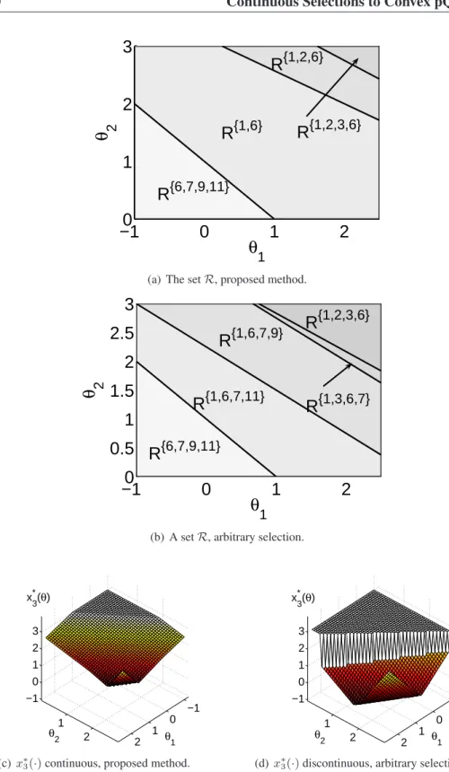
Our main motivation for obtaining continuous solutions to convex pQPs, be-sides the theoretical aspects, is that this problem arises in explicit model predictive control with a linear cost function (Bemporad, Borrelli, and Morari 2002). It is illustrated in (Bemporad, Borrelli, and Morari 2002) that the solution to an MPC problem with a linear cost function may be discontinuous if the algorithm in (Bor-relli, Bemporad, and Morari 2003) is used. Discontinuities of the optimizer func-tion may lead to chattering in an optimal control approach, and hence, a method which yields a continuous optimizer function is desirable. A unique representa-tion also gives benefits in terms ofi)Repeatability: The same solution is always obtained.ii)Parallelization: The parameter space can be divided into subsets that are explored individually without increasing the solution complexity when the re-sults are merged.iii) Exploration strategy: We have some freedom in the choice of algorithm used to explore the parameter space.

This chapther is based on (Spjøtvold, Tøndel, and Johansen 2005a; Spjøtvold, Tøndel, and Johansen 2005b; Spjøtvold, Tøndel, and Johansen 2007) and is orga-nized as follows: We first point out that using the normal cone optimality condition to construct parametric regions of optimality for strictly convex pQPs (Mayne and Rakovi´c 2003) results in a unique collection of polyhedral sets. For convex pQPs a unique set of non-intersecting polyhedra is obtained by always choosing the op-timizer with the least Euclidian norm and using the normal cone optimality con-dition. If the pQP has non-unique solutions, a strictly convex pQP is formulated such that the norm of the solution vector is minimized subject to the optimality conditions of the original problem. We prove that if the optimal set mapping for the convex pQP is continuous, the minimum norm selection will be a continuous mapping from the feasible subset of the parameter space to the solution space.

2.2 Preliminaries

2.2.1 Notation and basic definitions

IfI is an index set, then |I|denotes the cardinality of I andIi refers to theith

element in I. When referring to a set of indices I, we assume that the set is ordered, i.e. for theith _{element in} _I _{we have} _I

i < Ij, ∀j ∈ {i+ 1, . . . ,|I|}.

IfA ∈ Rn×m _{is a matrix or column vector, then}_A

i ∈ R1×m denotes theith row

ofAandA_I ∈R|I|×m_{denotes the matrix}h_AT

I1, . . . , A

T

I|I|

i_T

. Iff :X →Y is a function, then the restriction off to the domainD⊆Xis writtenf|D :D→Y.

Theclosure,interior, andboundaryof a setSis denotedcl(S),int(S), andbd(S), respectively. The abbreviation s.t. will denotesubject to.

Recall that the set of affine combinations of points in a setS ⊂ Rn is called theaffine hullofS, and is denotedaff(S). Thedimension of a setS ⊂Rn_{is the}

(27)

2.2 Preliminaries 15

be full-dimensional. Apolyhedronis the intersection of a finite number of closed halfspaces. A non-empty setF is afaceof the polyhedronP ⊂Rnif there exists a hyperplane {z ∈ Rn _| _aT_z ₌ _b_}_{, where} _a _∈ _Rn_, _b _∈ _{R, such that} _F ₌

P ∩ {z ∈ Rn _| _aT_z ₌ _b_} _and_aT_z _≤ _b_{for all}_z _∈ _P_{. Given an}_s_-dimensional

polyhedronP ⊂ Rn, wheres ≤ n, thefacetsofP are the(s−1)-dimensional faces ofP.

2.2.2 Problem setup

The problem that will be considered is given by

J∗(θ) := min

x∈Rnf(x, θ) s.t. Ax≤b+Sθ, (2.1) where f(x, θ) := 1₂xT_Hx ₊_θT_FT_x ₊_cT_x_, _θ _∈ _Rs _{is the} _parameter _{of the}

optimization problem, and the vector x ∈ Rn _{is to be optimized for all values}

ofθ∈Θ, whereΘ⊆Rs_{is a polyhedral set such that the minimum in (2.1) exists.}

Moreover,H=HT _∈_Rn×n_,_F _∈_Rn×s_,_A_∈_Rq×n_,_b_∈_Rq×1_and_S _∈_Rq×s_{. If}

in addition,H ≥0orH >0, the pQP is convex or strictly convex, respectively. IfH = 0, then (2.1) is a special form of parametric linear programs (pLP), which is a subclass of the problem addressed in this chapter. The point-to-set mapsX : Θ→ 2Rn

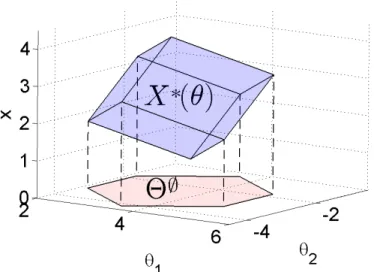
andX∗ _{: Θ} _→ ₂Rn

are defined asX(θ) := {x∈Rn _|_Ax_≤_b₊_Sθ_}

andX∗(θ) :={x∈Rn|Ax≤b+Sθ, f(x, θ) =J∗(θ)}, respectively. The sets

X(θ)andX∗₍_θ₎_{are referred to as the}_feasible_{- and}_{optimal set}_{, respectively.} Without loss of generality, the following standing assumption is made (Bempo-rad, Morari, Dua, and Pistikopoulos 2002; Borrelli, Bempo(Bempo-rad, and Morari 2003):

Assumption 2.1 The set of admissible parametersΘis full-dimensional.

Definition 2.1 (Active set) Letx be a feasible point of (2.1) for a givenθ. The

active constraints are the constraints that fulfill A_ix −b_i −S_iθ = 0, and the

inactive constraintsare the constraints that fulfillAix−bi−Siθ <0. Theactive

setA(x, θ)is the set of indices of the active constraints, that is, A(x, θ) :={i∈ {1,2, . . . , q}|Aix−bi−Siθ= 0}.

Definition 2.2 (Optimal active set) Letθbe given. Theoptimal active setA∗₍_θ₎ is the set of indices of the constraints that are active for allx∈X∗₍_θ₎_{, that is,}

A∗(θ) :={i|i∈ A(x, θ),∀x∈X∗(θ)}= \

x∈X∗₍_θ₎

A(x, θ).

Definition 2.3 (Critical region) Given an index setA ⊆ {1,2, . . . , q}, the critical regionΘA_{associated with}_A_{is the set of parameters for which the optimal active} set is equal toA, i.e.

(28)

16 Continuous Selections to Convex pQPs

In the above definition, note that if A is not the optimal active set for some parameter, thenΘA is the empty set. Hence, when referring to a critical region ΘA_{, we will assume that}_A_{is the optimal active set for some}_θ_∈_Θ_.

Definition 2.4 (LICQ) For a non-empty index setA ⊆ {1,2, . . . , q}, we say that the linear independence constraint qualification (LICQ) holds forAif the gradi-ents of the set of constraints indexed byAare linearly independent, i.e.AA has full row rank.

The following was established in (Bemporad, Morari, Dua, and Pistikopoulos 2002; Tøndel, Johansen, and Bemporad 2003c):

Theorem 2.1 (Solution properties) Consider the pQP in(2.1).

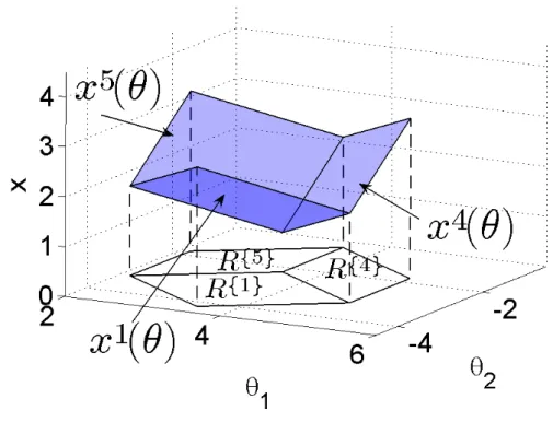
i) There exists a minimizer functionx∗ _{: Θ} _→ _Rn_,_θ _7→ _x∗₍_θ₎ _∈ _X∗₍_θ₎_{, that} is piecewise affine (PWA) in the sense that there exists a finite set of full-dimensional polyhedraR:={R1_{, . . . , R}K_}_{such that}_{Θ =}_∪K

k=1Rk,int(Ri)∩ int(Rj_{) =} _∅ _{for all}_i ₆₌ _j _{and the restriction} _x∗_|

Rk(·)is affine for all k ∈

{1, . . . , K}.

ii) The value functionJ∗_{: Θ}_→_R_{is continuous and piecewise quadratic (PWQ)} in the sense that the restrictionJ∗_|

Rk(·)is quadratic for allRk∈ R.

In the sequel we letx∗_∈_X∗₍_θ₎_{denote a minimizer to (2.1) for a given}_θ_,_x∗₍_·₎ denotes a piecewise affine selection function, andx∗₍_θ₎ _denotes_x∗₍_·₎ _evaluated atθ.

Our main objective is to obtain a unique set of full-dimensional polyhedraR

and simultaneously ensure that the functionx∗(·) is continuous. Thus, givenθ ∈

Θ, we will first consider how to select the affine restriction x∗_|

Rk(·)and find its polyhedral domain Rk_{. A polyhedral domain}_Rk _{∈ R}_{will be referred to as a} sub-regionsince in subsequent sections it will become apparent that eachRkmust be contained in the closure of a critical region. For the purpose of computing the domainRk_{, the next section summarizes the normal cone optimality condition.}

2.2.3 Normal cone optimality condition

Recall that a set C is called a cone if for every x ∈ C and scalar ξ ≥ 0, we haveξx ∈C. Moreover, a cone represented by the intersection of a finite number of closed half-spaces is called an H-cone, and the set of all nonnegative com-binations of a set of vectors {v1, . . . , vn} is called a V-cone. If A is a matrix,

then cone(A) denotes the set of all nonnegative combinations (V-cone) of the column-vectors ofA.

Consider the following problem:

z∗ := min

x∈Rnf(x) s.t. x∈Ω,

(29)

2.2 Preliminaries 17

where f(·),g_i(·) and h_j(·) are smooth, real-valued, functions defined on a sub-set of Rn and the index setsI andJ contain a finite number of elements. The following definitions are taken from (Nocedal and Wright 1999):

Definition 2.5 (Tangent and Normal cones) i) A vectorw∈Rn_{is tangent to}_Ω atx∈Ωif for all vector sequences{xi}withxi→xandxi ∈Ω, and all pos-itive scalar sequencest_i ↓0, there is a sequencew_i →wsuch thatx_i+t_iw_i ∈

Ωfor alli.

ii) The tangent coneTΩ₍_x₎_{is the collection of all tangent vectors to}_Ω_at_x_.

iii) The normal cone toΩatx,NΩ(x), is the orthogonal complement of the tan-gent cone, that is

Theorem 2.2 (First order necessary optimality condition) Ifx¯ is a local mini-mizer off inΩ, then

−∇_xf(¯x)∈NΩ(¯x). (2.2)

PROOF: See (Nocedal and Wright 1999).

Iff(·)andΩare convex, thenx¯is a global minimum and (2.2) is also sufficient. Given the polyhedron P := {x|Ax ≤ b}, letx¯ be a point on the boundary ofP. LetAbe the non-empty set of indices of the inequalities that are active atx¯, henceAix¯=bifori∈ A, andAix < b¯ ifori /∈ A. Note that for a polyhedron the

tangent coneTP_(¯_x₎_at_x_¯_{, is equal to the set of feasible directions at}_x_¯_(Bertsekas,

Nedic, and Ozdaglar 2003), i.e.TP_(¯_x_{) :=}_{_d_|_A

Ad≤0}. The normal cone atx¯is theV-coneNP_(¯_x_{) =}_cone₍_AT

A). TheH-cone representingNP(¯x)can always be written as

NP(¯x) ={y |LIy≤0, LEy = 0},

whereLI (LE) is a matrix representing the inequality (equality) part of the cone.

Iy≤0, LAEy= 0

ª

=NP_(¯_x₎_{. The optimality}

con-dition (2.2) becomes

L_I∇_xf(¯x)≥0, LE∇xf(¯x) = 0.

2.2.4 Continuity properties of solutions to pQPs

Before we introduce the minimum norm selection method, we consider the con-tinuity properties of the optimal set mapping for a convex pQP. For convenience we recall Berge’s definitions of a continuous, upper semicontinuous, and lower semicontinuous point-to-set map (Berge 1963):

(30)

18 Continuous Selections to Convex pQPs Definition 2.6 (Upper and lower semicontinuous point-to-set map) The point-to-set mapP :X →Y islower semicontinuousatx0, if for each open setΩ

satisfy-ingΩ∩P(x0)=6 ∅there is a neighborhoodU(x0)such that

x∈U(x0)⇒P(x)∩Ω6=∅.

Moreover,Pis lower semicontinuous onXif it is lower semicontinuous at eachx∈

X.

The point-to-set mapP : X → Y isupper semicontinuousatx₀, if for each open setΩcontainingP(x0)there exists a neighborhoodU(x0)such that

x∈U(x₀)⇒P(x)⊂Ω.

Moreover,Pis upper semicontinuous onXif it is upper semicontinuous at eachx∈

X.

Definition 2.7 (Continuous point-to-set map) The point-to-set mapP :X→Y

is continuous atx₀ if it is both upper semicontinuous and lower semicontinuous atx0. It is continuous onXif and only if it is continuous at everyx∈X.

Theorem 2.3 Consider problem (2.1) and let the point-to-set mapX∗₍_·₎_be con-tinuous onΘ. The PWA selection functionx∗₍_·₎_{with the least Euclidean norm is} continuous onΘ.

PROOF: It is obvious that the problem of finding the minimum norm solution can be stated as:

min

x∈Rn 1 2x

T_x _s.t. _x_∈_X∗₍_θ₎_.

The minimizer of a strictly convex function over a continuous point-to-set map is a continuous function (Berge 1963, Theorem VI.3.3), (Aubin and Frankowska 1990, Corollary 9.3.3).

¤

Since the existence of a continuous selection for problem (2.1) is ensured by the continuity of X∗₍_·₎ _on _Θ _{we state the following corollary based on (Bank,} Guddat, Klatte, Kummer, and Tammer 1983, Theorem 3.2.2, Theorem 3.2.3, and Theorem 5.3.2), which shows thatX∗(·)is in fact continuous in some cases.

Corollary 2.1 Consider problem (2.1). The point-to-set mapX∗(·)is continuous onΘif

i)

∀θ∈Θ@d∈Rn\{0}:Hd= 0∧ (c+F θ)Td= 0,

or

(31)

2.3 Strictly Convex pQP 19 PROOF: Note first that X∗₍_·₎ _{is upper semicontinuous on} _Θ _{(Bank, Guddat,} Klatte, Kummer, and Tammer 1983, Theorem 5.3.2).

i) By (Bank, Guddat, Klatte, Kummer, and Tammer 1983, Theorem 3.2.3)X∗₍_·₎ is lower semicontinuous onΘif the lineality space

M(θ) :={d∈Rn|Hd= 0,(c+F θ)Td= 0, A_A∗₍_θ₎d= 0} has the same dimension∀θ∈Θ. Ifi)holds, thendim(M(θ)) = 0,∀θ∈Θ.

ii) It follows from (Bank, Guddat, Klatte, Kummer, and Tammer 1983, Theorem 3.2.2 and page 47) that if X∗(θ)can be written as

{x∈Rn |gi(x, θ) :=hi(x) +ti(θ)≤0, i∈ I }

where for alli∈ I the functionshi(·)are convex onRn,ti(·)are continuous onΘ, andgi(·,·)are continuous onRn×Θ, thenX∗(·)is lower semicontin-uous onΘ. This is clearly the case for

X∗(θ) := ½ x∈Rn ¯ ¯ ¯ ¯Ax≤b+Sθ,1₂xTHx+cTx≤J∗(θ) ¾ . ¤ Remark 2.1 One (informal) way of interpreting conditioni)of Corollary 2.1 is that there does not exist a value forx(apart fromx = 0) for which the objective function vanishes and at the same time some perturbation ofθwill yield a positive objective function, while some other perturbation renders it negative. Looking at conditioni)in conjunction with the proof we see that the condition is sufficient and not necessary. A less restrictive condition is listed in the proof, however, it is much harder to check in practice as it must be checked for all optimal active sets.

2.3 Strictly Convex pQP

In this section we emphasize that for strictly convex pQPs a unique set of poly-hedraR can be found simply by identifying the closures of the full-dimensional critical regions. If H > 0 in (2.1), the problem can be recast such that only a quadratic term remains in the objective function (Bemporad, Morari, Dua, and Pis-tikopoulos 2002). Without loss of generality, we use the following formulation for strictly convex pQP J∗(θ) := min x∈Rn 1 2x T_Hx _s.t. _Ax_≤_b₊_Sθ. _(2.3)

The following corollary was established in (Bemporad, Morari, Dua, and Pis-tikopoulos 2002):

(32)

20 Continuous Selections to Convex pQPs Corollary 2.2 (Corollary to Theorem 2.1) The PWA minimizer functionx∗_{: Θ}_→ Rnto(2.3)is continuous.

A method for computing the expression for the restrictionx∗_|

Rk(·)and its polyhe-dral domainRkis summarized below. The KKT conditions for (2.3) are:

Hx+ATλ= 0, λ∈Rq,

λi(Aix−bi−Siθ) = 0, ∀i∈ {1, . . . , q},

Ax−b−Sθ≤0,

λi≥0, ∀i∈ {1, . . . , q},

whereλare the Lagrange multipliers. Assume that an index setAis given such that it is an optimal active set for some parameterθ∈Θand letN :={1,2, . . . , q}\A. If LICQ holds for A, then the KKT conditions can be manipulated (Bemporad, Morari, Dua, and Pistikopoulos 2002) to obtain the following two affine functions:

xA(θ) :=−H−1AT_AλA(θ),

λA(θ) :=−(AAH−1ATA)−1(bA+SAθ). IfRk_{is the closure of the critical region associated with}_A_{, i.e.}

Rk:= cl(ΘA) = ½ θ∈Θ ¯ ¯ ¯ ¯ ANx A₍_θ₎_≤_b N +SNθ λA(θ)≥0 ¾ ,

then the restriction of the minimizer functionx∗₍_·₎_{to the polyhedron}_Rk_{is given}

by x∗|_Rk(θ) = xA(θ). However, if LICQ is violated for A, the normal cone optimality condition can be used as proposed in (Mayne and Rakovi´c 2003); the affine functionxA₍_·₎_{is defined as the (unique) solution to}

· LA EH AA ¸ x= · 0 bA ¸ + · 0 SA ¸ θ. (2.4)

In (Mayne and Rakovi´c 2003) the following was established:

Theorem 2.4 (Closure of a critical region) The minimizer function xA₍_·₎_, asso-ciated with the optimal active setA, which is defined as the solution to(2.4), is optimal in the polyhedron defined by

RA:= cl¡ΘA¢= ½ θ∈Θ ¯ ¯ ¯ ¯ ANx A₍_θ₎_≤_b N +SNθ LA IHxA(θ)≥0 ¾ , (2.5) whereLA

I is the inequality part of a representation of the normal cone defined by the optimal active setAandN :={1, . . . , q}\A.

PROOF: See (Mayne and Rakovi´c 2003).

(33)

2.4 Convex pQP 21

Thus, where it is clear from the context,Rk_{will refer to the}_kth _{set in}_R_and_RA will refer to the set inRassociated with the optimal active setA.

Remark 2.2 Note that since the setRAis constructed using optimality conditions, we do not treat the cases whereA∗₍_θ_{) =} _∅_or_A∗₍_θ_{) =} _{₁_{, . . . , q}_} _{explicitly. It} should be apparent that we do not need to demand the solution feasible ifA∗₍_θ_{) =}

{1, . . . , q}, and there is no equationAA = bA +SAθ that needs to be satisfied ifA=A∗₍_θ_{) =}_∅_.

For a strictly convex pQP the functionx∗₍_·₎_{is then defined as}

x∗(θ) :=xA(θ) if θ∈RA, (2.6) and the collectionRin Theorem 2.1 becomes

Corollary 2.3 (Uniqueness of the solution) For a strictly convex pQP, the collec-tion R obtained by defining sub-regions as in (2.5), is unique and satisfies the properties in Theorem 2.1.

PROOF: Uniqueness ofRA _{follows directly from uniqueness of the optimal} active setA,xA₍_θ₎_{, and the normal cone}_NX(θ)₍_x∗₍_θ₎₎_{for all}_θ_∈_Θ_{. All}_RA _∈

R are closures of critical regions, and since critical regions do not intersect,

int¡Ri¢_∩_int¡_Rj¢ ₌ _∅_,_i ₆₌ _j_{. Since the number of optimal active sets is} fi-nite,∪K

k=1Rk= Θtrivially holds.

¤

2.4 Convex pQP

Consider problem (2.1). In the rest of the chapterHis only restricted to be posi-tive semi-definite and symmetric (this includesH = 0). Compared to the strictly convex case, a number of difficulties arise with regards to obtaining a unique setR

and a c