Programming the K-means Clustering Algorithm in SQL
Carlos Ordonez
Teradata, NCR
San Diego, CA 92127, USA
ABSTRACT
Using SQL has not been considered an efficient and feasible way to implement data mining algorithms. Although this is true for many data mining, machine learning and statistical algorithms, this work shows it is feasible to get an efficient SQL implementation of the well-known K-means clustering algorithm that can work on top of a relational DBMS. The article emphasizes both correctness and performance. From a correctness point of view the article explains how to com-pute Euclidean distance, nearest-cluster queries and updat-ing clusterupdat-ing results in SQL. From a performance point of view it is explained how to cluster large data sets defining and indexing tables to store and retrieve intermediate and final results, optimizing and avoiding joins, optimizing and simplifying clustering aggregations, and taking advantage of sufficient statistics. Experiments evaluate scalability with synthetic data sets varying size and dimensionality. The proposed K-means implementation can cluster large data sets and exhibits linear scalability.
Categories and Subject Descriptors
H.2.8 [Database Management]: Database Applications-Data Mining
General Terms
Algorithms, Languages
Keywords
Clustering, SQL, relational DBMS, integration
1. INTRODUCTION
There exist many efficient clustering algorithms in the data mining literature. Most of them follow the approach proposed in [14], minimizing disk access and doing most of the work in main memory. Unfortunately, many of those al-gorithms are hard to implement inside a real DBMS where
Permission to make digital or hard copies of all or part of this work for personal or classroom use is granted without fee provided that copies are not made or distributed for profit or commercial advantage and that copies bear this notice and the full citation on the first page. To copy otherwise, to republish, to post on servers or to redistribute to lists, requires prior specific permission and/or a fee.
KDD’04,August 22–25, 2004, Seattle, Washington, USA. Copyright 2004 ACM 1-58113-888-1/04/0008 ...$5.00.
the programmer needs to worry about storage management, concurrent access, memory leaks, fault tolerance, security and so on. On the other hand, SQL has been growing over the years to become a fairly comprehensive and complex query language where the aspects mentioned above are au-tomatically handled for the most part or they can be tuned by the database application programmer. Moreover, nowa-days SQL is the standard way to interact with a relational DBMS. So can SQL, as it exists today, be used to get an effi-cient implementation of a clustering algorithm? This article shows the answer is yes for the popular K-means algorithm. It is worth mentioning programming data mining algorithms in SQL has not received too much attention in the database literature. This is because SQL, being a database language, is constrained to work with tables and columns, and then it does not provide the flexibility and speed of a high level pro-gramming language like C++ or Java. Summarizing, this article presents an efficient SQL implementation of the K-means algorithm that can work on top of a relational DBMS to cluster large data sets.
The article is organized as follows. Section 2 introduces definitions and an overview of the K-means algorithm. Sec-tion 3 introduces several alternatives and optimizaSec-tions to implement the K-means algorithm in SQL. Section 4 con-tains experiments to evaluate performance with synthetic data sets. Section 5 discusses related work. Section 6 pro-vides general conclusions and directions for future work.
2. DEFINITIONS
The basic input for K-means [2, 6] is a data setY contain-ing n points ind dimensions, Y ={y1, y2, . . . , yn}, andk,
the desired number of clusters. The output are three matri-cesW, C, R, containingkweights,k means andkvariances respectively corresponding to each cluster and a partition of
Y intoksubsets. MatricesCandRared×kandW isk×1. Throughout this work three subscripts are used to index ma-trices: i= 1, . . . , n, j= 1, . . . , k, l= 1, . . . , d. To refer to one column ofC or R we use thej subscript (e.g. Cj, Rj); Cj
can be understood as ad-dimensional vector containing the centroid of thejth cluster having the respective squared ra-diuses per dimension given byRj. For transposition we will use theTsuperscript. For instanceCj refers to thejth cen-troid in column form andCT
j is thejth centroid in row form.
LetX1, X2, . . . , Xkbe theksubsets ofY induced by clusters
s.t. Xj ∩Xj0 =∅, j6=j
0
. K-means uses Euclidean distance to find the nearest centroid to each input point, defined as
d(yi, Cj) = (yi−Cj)T(yi−Cj) =Pd
l=1(yli−Clj) 2
. K-means can be described at a high level as follows.
Cen-troids Cj are generally initialized with k points randomly selected fromY for an approximation when there is an idea about potential clusters. The algorithm iterates executing the E and the M steps starting from some initial solution un-til cluster centroids become stable. The E step determines the nearest cluster for each point and adds the point to it. That is, the E step determines cluster membership and par-titionsY intoksubsets. The M step updates all centroidsCj
by averaging points belonging to the same cluster. Then the
k cluster weights Wj and thekdiagonal variance matrices
Rj are updated based on the newCj centroids. The quality of a clustering solution is measured by the average quantiza-tion errorq(C) (also known as squared assignment distance [6]). The goal of K-means is minimizing q(C), defined as
q(C) = Pni=1d(yi, Cj)/n. where yi ∈ Xj. This quantity
measures the average squared distance from each point to the cluster where it was assigned according to the parti-tion intoksubsets. K-means stops whenq(C) changes by a marginal fraction () in consecutive iterations. K-means is theoretically guaranteed to converge decreasingq(C) at each iteration [6], but it is common to set a maximum number of iterations to avoid long runs.
3. IMPLEMENTING K-MEANS IN SQL
This section presents our main contributions. We explain how to implement K-means in a relational DBMS by auto-matically generating SQL code given an input tableY with
dselected numerical columns andk, the desired number of clusters as input as defined in Section 2. The SQL code gen-erator dynamically creates SQL statements monitoring the difference of quality of the solution in consecutive iterations to stop. There are two main schemes presented in here. The first one presents a simple implementation of K-means ex-plaining how to program each computation in SQL. We refer to this scheme as the Standard K-means implementation. The second scheme presents a more complex K-means im-plementation incorporating several optimizations that dra-matically improve performance. We call this scheme the Optimized K-means implementation.
There are important assumptions behind our proposal from a performance point of view. Two tables withn rows having the same primary key can be joined in time O(n) using a hash-based join. So if a different DBMS does not provide hash-based indexing, joining tables may take longer thanO(n). However, the proposed scheme should still pro-vide the most efficient implementation even in such cases. In general it is assumed that n is large, whereas d and k
are comparatively small. This has a direct relationship to how tables are defined and indexed, and to how queries are formulated in SQL. These assumptions are reasonable in a database environment.
3.1 Basic Framework
The basic scheme to implement K-means in SQL, having
Y andkas input (see Section 2), follows these steps: 1. Setup. Create, index and populate working tables. 2. Initialization. InitializeC.
3. E step. Computekdistances per pointyi. 4. E step. Find closest centroidCj to each pointyi. 5. M step. UpdateW, C andR.
6. M step. Update table to track K-means progress. Steps 3-6 are repeated until K-means converges.
3.2 Standard K-means
Creating and populating working tables
In the following paragraphs we discuss table definitions, in-dexing and several guidelines to write efficient SQL code to implement K-means. In general we omit Data Defini-tion Language (DDL) statements and deleDefini-tion statements to make exposition more concise. Thus most of the SQL code presented involves Data Manipulation Language (DML) state-ments. The columns making up the primary key of a table are underlined. Tables are indexed on their primary key for efficient join access. Subscriptsi, j, l(see Section 2) are de-fined as integer columns and thednumerical dimensions of points ofY, distances, and matrix entries ofW, C, Rare de-fined as FLOAT columns in SQL. Before each INSERT state-ment it is assumed there is a ”DELETE FROM ... ALL;” statement that leaves the table empty before insertion.
As introduced in Section 2 the input data set has d di-mensions. In database terms this means there exists a table Y with several numerical columns out of whichd columns are picked for clustering analysis. In practice the input ta-ble may have many more than d columns but to simplify exposition we will assume its definition is Y(Y1, Y2, .., Yd).
So the SQL implementation needs to build its own reduced version projecting the desired d columns. This motivates defining the following ”horizontal” table withd+ 1 columns:
Y H(i, Y1, Y2, ..., Yd) havingias primary key. The first
col-umn is theisubscript for each point and thenY Hhas the list ofddimensions. This table saves Input/Output access (I/O) since it may have fewer columns than Y and it is scanned several times during the algorithm progress. In general it is not guaranteedi(point id) exists because the primary key ofY may consist of more than one column, or it may not exist at all becauseY is the result of some aggrega-tions. In an implementation in an imperative programming language like C++ or Java the point identifier is immaterial sinceY is accessed sequentially, but in a relational database it is essential. Therefore it is necessary to automatically create iguaranteeing a unique identifier for each point yi. The following statement computes a cumulative sum on one scan over Y to geti∈ {1. . . n}and projects the desiredd
columns.
INSERT INTO YH
SELECT sum(1) over(rows unbounded preceding) AS i ,Y1, Y2, . . . , Yd
FROMY;
The point identifier ican be generated with some other SQL function than returns a unique identifier for each point. Getting a unique identifier using a random number is not a good idea because it may get repeated, specially for very large data sets. As seen in Section 2 clustering results are stored in matricesW, C, R. This fact motivates having one table for each of them storing one matrix entry per row to allow queries access each matrix entry by subscripts j
and l. So the tables are as follows: W(j, w), C(l, j, val),
R(l, j, val), havingk,dkanddk rows respectively.
The table Y H defined above is useful to seed K-means, but it is not adequate to compute distances using the SQL ”sum()” aggregate function. So it has to be transformed into a ”vertical” table having d rows for each input point, with one row per dimension. This leads to tableY V with
definitionY V(i, l, val). Then tableY V is populated withd
statements as follows:
INSERT INTO YV SELECT i,1,Y1 FROM YH; . . .
INSERT INTO YV SELECT i,d,Yd FROM YH;
Finally we define a table to store several useful numbers to track K-means progress. Table model serves this purpose:
model(d, k, n, iteration, avg q, dif f avg q).
Initializing K-means
Most K-means variants usekpoints randomly selected from
Y to seed C. Since W and R are output they do not re-quire initialization. In this case Y H proves adequate for this purpose to seed a ”horizontal” version of C. Table
CH(j, Y1, . . . , Yd) is updated as follows.
INSERT INTO CH
SELECT 1,Y1, .., YdFROM YH SAMPLE 1; . . .
INSERT INTO CH
SELECT k,Y1, .., YdFROM YH SAMPLE 1;
OnceCH is populated it can be used to initializeCwith
dk statements as follows, INSERT INTO C
SELECT 1,1, Y1FROM CH WHEREj= 1; . . .
INSERT INTO C
SELECTd, k, Yd FROM CH WHEREj=k;
Computing Euclidean distance
K-means determines cluster membership in the E step. This is an intensive computation since it requiresO(dkn) oper-ations. Distance computation needs Y V and C as input . The output should be stored in a table having k dis-tances per point. That leads to the table Y D defined as
Y D(i, j, distance). The SQL is as follows. INSERT INTO YD
SELECTi, j,sum((YV.val-C.val)**2)
FROMY V, C WHEREY V.l=C.l GROUP BYi, j;
After the insertionY Dcontainsknrows. Before doing the GROUP BY there is an intermediate table with dknrows. This temporary table constitutes the largest table required by K-means.
Finding the nearest centroid
The next step involves determining the nearest neighbor (among clusters) to each point based on the k distances and storing the index of that cluster in table Y N N(i, j). Therefore, table Y N N will store the partition ofY into k
subsets being j the partition subscript. This requires two steps in SQL. The first step involves determining the mini-mum distance. The second step involves assigning the point to the cluster with minimum distance. A derived table and a join are required in this case. Table Y N N contains the partition of Y and will be the basic ingredient to compute centroids. This statement assumes that the minimum dis-tance is unique for each point. In abnormal cases, where distances are repeated (e.g. because of repeated centroids, or many repeated points) ties are broken in favor of the cluster with the lowest subscriptj; that code is omitted.
INSERT INTOY N N
SELECTY D.i, Y D.j
FROMY D, (SELECTi, min(distance) AS mindist FROM YD GROUP BYi)YMIND
WHEREY D.i=Y M IN D.i
andY D.distance=Y M IN D.mindist;
Updating clustering results
The M step updates W, C, Rbased on the partitionY N N
obtained in the E step. Given the tables introduced above updating clustering parameters is straightforward. The SQL generator just needs to count points per cluster, compute the average of points in the same cluster to get new centroids, and compute variances based on the new centroids. The respective statements are shown below.
INSERT INTOW SELECTj,count(*)
FROMY N NGROUP BYj;
UPDATEW SETw=w/model.n; INSERT INTOC
SELECTl, j, avg(Y V.val) FROMY V, Y N N
WHEREY V.i=Y N N.iGROUP BYl, j; INSERT INTOR
SELECTC.l, C.j,avg( (Y V.val−C.val)∗ ∗2) FROMC, Y V, Y N N
WHEREY V.i=Y N N.i
andY V.l=C.landY N N.j=C.j
GROUP BYC.l, C.j;
Observe that the M step as computed in SQL has com-plexity O(dn) because Y N N has n rows and Y V has dn
rows. That is, the complexity is notO(dkn), which would be the time required for a soft partition approach like EM. This fact is key to a better performance.
Finally, we just need to track K-means progress: UPDATE model
FROM (SELECT sum(W∗R.val) ASavg q
FROMR, W WHERER.j=W.j)avgR
SETavg q=avgR.avg q,iteration=iteration+1;
3.3 Optimized K-means
Even though the implementation introduced above cor-rectly expresses K-means in SQL there are several optimiza-tions that can be made. These optimizaoptimiza-tions go from physi-cal storage organization and indexing to concurrent process-ing and exploitprocess-ing sufficient statistics.
Physical storage and indexing of large tables
We now discuss how to index tables to provide efficient ac-cess and improve join performance. TablesY H(i, Y1, .., Yd)
andY N N(i, j) havenrows each, each hasias its primary key and both need to provide efficient join processing for points. Therefore, it is natural to index them on their pri-mary keyi. When one row ofY His accessed alldcolumns are used. Therefore, it is not necessary to individually index any of them. TableY V(i, l, val) hasdn rows and needs to provide efficient join processing withCto compute distances and with Y N N to update W, C, R. When K-means com-putes distances squared differences (yli−Clj)2
are grouped byiandj, beingithe most important factor from the per-formance point of view. To speed up processing all drows
corresponding to each point i are physically stored on the same disk block andY V has an extra index oni. The table block size for Y V is increased to allow storage of all rows on the same disk block. The SQL to compute distances is explained below.
Faster distance computation
For K-means the most intensive step is distance computa-tion, which has time complexityO(dkn). This step requires both significant CPU use and I/O. We cannot reduce the number of arithmetic operations required since that is in-trinsic to K-means itself (although under certain constraints computations may be accelerated), but we can optimize dis-tance computation to decrease I/O. Recalling the SQL code given in Section 3.2 we can see distance computation re-quires joining one table with dn rows and another table withdkrows to produce a large intermediate table withdkn
rows (call itY kdn). Once this table is computed the DBMS groups rows intodkgroups. So a critical aspect is being able to compute thekdistances per point avoiding this huge in-termediate tableY dkn. A second aspect is determining the nearest cluster givenkdistances fori∈1. . . n. Determining the nearest cluster requires a scan onY D, readingknrows, to get the minimum distance per point, and then a join to determine the subscript of the closest cluster. This requires joiningknrows withnrows.
To reduce I/O we propose to compute the k distances ”in parallel” storing them as k columns ofY D. Then the new definition for tableY DisY D(i, d1, d2, . . . , dk) with
pri-mary key i, wheredj =d(yi, Cj), the distance from point
i to thejth centroid. This decreases I/O since disk space is reduced (less space per row, index on n rows instead of
knrows) and thek distances per point can be obtained in one I/O instead ofkI/Os. This new scheme requires chang-ing the representation of matrixC to have allk values per dimension in one row or equivalent, containing one cluster centroid per column, to properly compute distances. This leads to a join producing a table with onlyn rows instead ofknrows, and creating an intermediate table withdnrows instead ofdknrows. ThusCis stored in a table defined as
C(l, C1, C2, . . . , Ck), with primary keyl and indexed by l.
At the beginning of each E step columnCis copied from a tableW CRto tableC. TableW CRis related to sufficient statistics concepts and will be introduced later. The SQL to compute thekdistances is as follows:
INSERT INTO YD SELECTi
,sum((Y V.val−C.C1)**2) ASd1 . . .
,sum((Y V.val−C.Ck)**2) ASdk
FROMY V, C WHEREY V.l=C.lGROUP BYi;
Observe each dimension of each point in Y V is paired with the corresponding centroid dimension. This join is effi-ciently handled by the query optimizer becauseY V is large andC is small. An alternative implementation with UDFs, not explored in this work, would require to have a different distance UDF for each value of d, or a function allowing a variable number of arguments (e.g. the distance between
yi andCj would bedistance(y1i, C1j, y2i, C2j, . . . , ydi, Cdj).
This is because UDFs can only take simple data types (float-ing point numbers in this case) and not vectors. Efficiency would be gained by storing matrixC in cache memory and
avoiding the join. But a solution based on joins is more elegant and simpler and time complexity is the same.
Nearest centroid without join
The disadvantage about k distances being all in one row is that the SQLmin() aggregate function is no longer use-ful. We could transformY D into a table withknrows and then use the same approach introduced in Section 3.2 but that transformation and the subsequent join would be slow. Instead we propose to determine the nearest cluster using a CASE statement instead of calling the min() aggregate function. Then the SQL to get the subscript of the closest centroid is:
INSERT INTOY N N SELECTi, CASE
WHENd1 ≤d2 .. ANDd1≤dkTHEN 1
WHENd2 ≤d3 .. ANDd2≤dkTHEN 2 . . .
ELSEk
END FROMY D;
It becomes evident from this approach there is no join needed and the search for the closest centroid for one point is done in main memory. The nearest centroid is determined in one scan on Y D. Then I/O is reduced from (2kn+n) I/Os tonI/Os. Observe that thejth WHEN predicate has
k−jterms. That is, as the search for the minimum distance continues the number of inequalities to evaluate decreases. however, the CASE statement has time complexity O(k2
) instead of O(k) which is the usual time to determine the nearest centroid. So we slightly affect K-means performance from a theoretical point of view. But I/O is the main perfor-mance factor and this CASE statement works in memory. If
kis more than the maximum number of columns allowed in the DBMSY D andCcan be vertically partitioned to over-come this limitation. This code could be simplified with a User Defined Function ”argmin()” that returns the sub-script of the smallest argument. The problem is this function would require a variable number of arguments.
Sufficient Statistics
Now we turn our attention to how to accelerate K-means us-ing sufficient statistics. Sufficient statistics have been shown to be an essential ingredient to accelerate data mining al-gorithms [2, 4, 14, 7]. So we explore how to incorporate them into a SQL-based approach. The sufficient statistics for K-means are simple. Recall from Section 2 Xj repre-sents the set of points in clusterj. We introduce three new matricesN, M, Qto store sufficient statistics. MatrixN is
k×1, matrices M and Q are d×k. Observe their sizes are analogous toW, C, Rsizes and thatQj represents a di-agonal matrix analogous to Rj. Nj stores the number of points,Mj stores the sum of points andQj stores the sum of squared points in clusterjrespectively. ThenNj =|Xj|,
Mj =Py
i∈Xjyi,Qj =
P
yi∈Xjy T
iyi. Based on these three
equations W, C, R are computed as Wj = Nj/PkJ=1WJ, Cj =Mj/Nj,Rj =Qj/Nj−CT
j Cj.
To update parameters we need to join Y N N, that con-tains the partition ofY intoksubsets, withY V, that con-tains the actual dimension values. It can be observed that from a database point of view sufficient statistics allow mak-ing one scan over the partitionXj given byY N N grouped
byj. The important point is that the same statement can be used to update N, M, Q if they are stored in the same table. That is, keeping a denormalized scheme. So instead of having three separate tables, N, M, Qare stored on the same table. But if we keep sufficient statistics in one table that leads to also keeping the clustering results in one table. So we introduce table definitions: N M Q(l, j, N, M, Q) and
W CR(l, j, W, C, R). Both tables have the same structure and are indexed by the primary key (l, j). So these table definitions substitute the table definitions for the Standard K-means implementation introduced above. Then the SQL to update sufficient statistics is as follows:
INSERT INTON M QSELECT
l, j,sum(1.0) ASN
,sum(Y V.val) ASM ,sum(Y V.val*YV.val) ASQ
FROMY V, Y N N WHEREY V.i=Y N N.i
GROUP BYl, j;
By using tableN M Q the SQL code for the M step gets simplified and becomes faster to updateW CR.
UPDATEW CRSETW = 0; UPDATEW CRSET
W =N
,C=CASE WHENN >0 THENM/N ELSEC END ,R=CASE WHENN >0 THENQ/N−(M/N)∗ ∗2
ELSER END
WHEREN M Q.l=W CR.l ANDN M Q.j =W CR.j; UPDATE WCR SET W=W/model.n;
An INSERT/SELECT statement, although equivalent and more efficient, would eliminate clusters with zero points from the output. We prefer to explicitly show those clusters. The main advantages of using sufficient statistics compared Stan-dard K-means, is thatMandQdo not depend on each other and together withN they are enough to updateC, R (elim-inating the need to scan Y V). Therefore, the dependence betweenCandRis removed and both can be updated at the same time. Summarizing, Standard K-means requires one scan overY N N to getW and two joins betweenY N N and
Y V to getCandRrequiring in total three scans overY N N
and two scans over Y V. This requires reading (3n+ 2dn) rows. On the other hand, Optimized K-means, based on sufficient statistics, requires only one join and one scan over
Y N N and one scan over Y V. This requires reading only (n+dn) rows. This fact speeds up the process considerably. Table W CR is initialized with dk rows having columns
W, R set to zero and column C initialized withk random points taken fromCH. TableCHis initialized as described in Section 3.2. Then CH is copied to column C inW CR. At the beginning of each E stepW CR.C is copied to table
C so that tableC is current.
4. EXPERIMENTAL EVALUATION
Experiments were conducted on a Teradata machine. The system was an SMP (parallel Symmetric Multi-Processing) with 4 nodes, having one CPU each running at 800 Mhz, and 40 AMPs (Access Module Processors) running Teradata V2R4 DBMS. The system had 10 terabytes of available disk space. The SQL code generator was programmed in the Java language, which connected to the DBMS through the JDBC interface.
4.1 Running time varying problem sizes
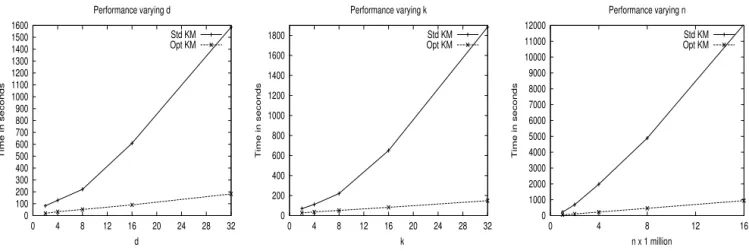
Figure 1 shows scalability graphs. We conducted our tests with synthetic data sets having defaults d= 8, k = 8, n = 1000k(with means in [0,10] and unitary variance) which rep-resent typical problem sizes in a real database environment. Since the number of iterations K-means takes may vary de-pending on initialization we compared the time for one itera-tion. This provides a fair comparison. The first graph shows performance varyingd, the second graph shows scalability at differentkvalues and the third graph shows scalability with the most demanding parameter: n. These graphs clearly show several differences among our implementations. Opti-mized K-means is always the fastest. Compared to Standard K-means the difference in performance becomes significant as d, k, nincrease. For the largest d, k, n values Optimized means is ten orders of magnitude faster than Standard K-means. Extrapolating these numbers, we can see Optimized K-means is 100 times faster than Standard K-means when
d= 32,k= 32 andn= 1M (ord= 32,k = 8,n= 16M) and 1000 times faster whend= 32,k= 32 andn= 16M.
5. RELATED WORK
Research on implementing data mining algorithms using SQL includes the following. Association rules mining is ex-plored in [12] and later in [5]. General data mining primi-tives are proposed in [3]. Primiprimi-tives to mine decision trees are introduced in [4, 13]. Programming the more powerful EM clustering algorithm in SQL is explored in [8].
Our focus was more on the side of writing efficient SQL code to implement K-means rather than proposing another ”fast” clustering algorithm [1, 2, 14, 9, 7]. These algorithms require a high level programming language to access memory and perform complex mathematical operations. The way we exploit sufficient statistics is similar to [2, 14]. This is not the first work to explore the implementation of a cluster-ing algorithm in SQL. Our K-means proposal shares some similarities with the EM algorithm implemented in SQL [8]. This implementation was later adapted to cluster gene data [11], with basically the same approach. We explain impor-tant differences between the EM and K-means implemen-tations in SQL. K-means is an algorithm strictly based on distance computation, whereas EM is based on probability computation. This results in a simpler SQL implementa-tion of clustering with wider applicability. We explored the possibility of using sufficient statistics in SQL, which are crucial to improve performance. The clustering model is stored in a single table, as opposed to three tables. Sev-eral aspects related to table definition, indexing and query optimization not addressed before are now studied in de-tail. A fast K-means prototype to cluster data sets inside a relational DBMS using disk-based matrices is presented in [10]. The disk-based implementation and the SQL-based implementation are complementary solutions to implement K-means in a relational DBMS.
6. CONCLUSIONS
This article introduced two implementations of K-means in SQL. The proposed implementations allow clustering large data sets in a relational DBMS eliminating the need to ex-port or access data outside the DBMS. Only standard SQL was used; no special data mining extensions for SQL were needed. This work concentrated on defining suitable
ta-0 100 200 300 400 500 600 700 800 900 1000 1100 1200 1300 1400 1500 1600 0 4 8 12 16 20 24 28 32 Time in seconds d Performance varying d Std KM Opt KM 0 200 400 600 800 1000 1200 1400 1600 1800 0 4 8 12 16 20 24 28 32 Time in seconds k Performance varying k Std KM Opt KM 0 1000 2000 3000 4000 5000 6000 7000 8000 9000 10000 11000 12000 0 4 8 12 16 Time in seconds n x 1 million Performance varying n Std KM Opt KM
Figure 1: Time per iteration varyingd, k, n. Defaults: d= 8, k= 8, n= 10 000,000
bles, indexing them and writing efficient queries for clus-tering purposes. The first implementation is a naive trans-lation of K-means computations into SQL and serves as a framework to introduce an optimized version with superior performance. The first implementation is called Standard K-means and the second one is called Optimized K-means. Optimized K-means computes all Euclidean distances for one point in one I/O, exploits sufficient statistics and stores the clustering model in a single table. Experiments evaluate performance with large data sets focusing on elapsed time per iteration. Standard K-means presents scalability prob-lems with increasing number of clusters or number of points. Its performance graphs exhibit nonlinear behavior. On the other hand, Optimized K-means is significantly faster and exhibits linear scalability. Several SQL aspects studied in this work have wide applicability for other distance-based clustering algorithms found in the database literature.
There are many issues that deserve further research. Even though we proposed an efficient way to compute Euclidean distance there may be more optimizations. Several aspects studied here also apply to the EM algorithm. Clustering very high dimensional data where clusters exist only on pro-jections of the data set is another interesting problem. We want to cluster very large data sets in a single scan using SQL combining the ideas proposed here with User Defined Functions, OLAP extensions, and more efficient indexing. Certain computations may warrant defining SQL primitives to be programmed inside the DBMS. Such constructs would include Euclidean distance computation, pivoting a table to have one dimension value per row and another one to find the nearest cluster given several distances. The rest of com-putations are simple and efficient in SQL.
7. REFERENCES
[1] C. Aggarwal and P. Yu. Finding generalized projected clusters in high dimensional spaces. InACM SIGMOD Conference, pages 70–81, 2000.
[2] P. Bradley, U. Fayyad, and C. Reina. Scaling clustering algorithms to large databases. InACM KDD Conference, pages 9–15, 1998.
[3] J. Clear, D. Dunn, B. Harvey, M.L. Heytens, and P. Lohman. Non-stop SQL/MX primitives for
knowledge discovery. InACM KDD Conference, pages 425–429, 1999.
[4] G. Graefe, U. Fayyad, and S. Chaudhuri. On the efficient gathering of sufficient statistics for
classification from large SQL databases. InACM KDD Conference, pages 204–208, 1998.
[5] H. Jamil. Ad hoc association rule mining as SQL3 queries. InIEEE ICDM Conference, pages 609–612, 2001.
[6] J.B. MacQueen. Some methods for classification and analysis of multivariate observations. InProc. of the 5th Berkeley Symposium on Mathematical Statistics and Probability, 1967.
[7] C. Ordonez. Clustering binary data streams with K-means. InACM DMKD Workshop, pages 10–17, 2003.
[8] C. Ordonez and P. Cereghini. SQLEM: Fast clustering in SQL using the EM algorithm. InACM SIGMOD Conference, pages 559–570, 2000.
[9] C. Ordonez and E. Omiecinski. FREM: Fast and robust EM clustering for large data sets. InACM CIKM Conference, pages 590–599, 2002.
[10] C. Ordonez and E. Omiecinski. Efficient disk-based K-means clustering for relational databases.IEEE TKDE, to appear, 2004.
[11] D. Papadopoulos, C. Domeniconi, D. Gunopulos, and S. Ma. Clustering gene expression data in SQL using locally adaptive metrics. InACM DMKD Workshop, pages 35–41, 2003.
[12] S. Sarawagi, S. Thomas, and R. Agrawal. Integrating mining with relational databases: Alternatives and implications. InACM SIGMOD Conference, 1998. [13] K. Sattler and O. Dunemann. SQL database
primitives for decision tree classifiers. InACM CIKM Conference, 2001.
[14] T. Zhang, R. Ramakrishnan, and M. Livny. BIRCH: An efficient data clustering method for very large databases. InACM SIGMOD Conference, pages 103–114, 1996.