Sample Images for Land Cover Studies.
Part 1: Methodology
J. Cihlar,
*
R. Latifovic,
*
J. Chen,
*
J. Beaubien,
†
and Z. Li
*
T
his is the first of two articles which explore the com- tained using the TM map. The performance of samples selected by a combination of cover composition and con-bined use of coarse and fine resolution data in land coverstudies. It describes the development and evaluation of tagion index responded to the characteristics of individ-ual tiles in terms of the selection criteria. A rigorous appli-an objective procedure to select a representative sample
of tiles of high resolution images that complements a cation of the algorithm with spatial heterogeneity measures such as the contagion index is computationally very de-coarse resolution coverage of an entire region of interest.
The second article explores the use of the procedure for manding. It is concluded that PSA provides an efficient and effective tool to select a representative sample for land an accurate estimation of cover type composition at the
regional scale. The Purposive Selection Algorithm (PSA) cover studies in which both large area coverage and local detail are desired. Elsevier Science Inc., 2000 assumes that a relationship exists between land cover
compositions at the two spatial scales. It selects one tile at a time, seeking the sample which most closely
resem-bles the composition of the coarse resolution map. Two INTRODUCTION
selection criteria were used, fraction of cover types and
The interest in land cover analysis at regional to global
contagion index. PSA was evaluated using two land cover
scales has grown dramatically in the last decade,
stimu-maps for a 288 km3165 km area in central
Saskatche-lated by global environmental change and by improved
wan, Canada derived from Landsat Thematic Mapper
mapping tools. The International Geosphere–Biosphere
images (30 m pixels) and Advanced Very High Resolution
Program (IGBP) identified a strong need for regional
Radiometer (AVHRR, 1000 m pixels), each divided into
and global land cover information (Townshend et al.,
64 tiles. The performance of an intermediate sensor (480
1994) to serve a variety of IGBP projects. Earlier work in
m pixels) was assessed by resampling the TM map. When
using NOAA AVHRR data for mapping land cover (e.g.,
using cover type composition alone, it was found that the
Loveland et al., 1991) led to the execution of a global 1
procedure rapidly converges on a representative set of
km data land cover mapping initiative formulated in
re-tiles with land cover composition very similar to the full
sponse to the IGBP and other requirements (Eidenshink
coverage. The match between the domain and sample
and Faundeen, 1994). Various regional studies have also
cover type fractions was very close, with errors less than
been undertaken, as were methodological studies to
im-0.002% once about 1/5 to 1/3 of the tiles were selected
prove land cover information extraction procedures over
and no discernible bias in the selected sample. Compared
large areas (e.g., Defries and Townshend, 1994; Belward,
to the TM whole area coverage, samples selected with
1996; Cihlar et al., 1996). As a result, quality land cover
AVHRR classification were as representative as those
ob-data sets over large terrestrial areas are emerging, and they will become reality with improved data sources such as provided by the MODIS instrument (Salomonson,
* Canada Centre for Remote Sensing, Ottawa, Ontario
† Canadian Forest Service, Quebec City, Quebec 1988) and planned new activities, for example, the Global Address correspondence to Josef Cihlar, Canada Centre for Re- Observation of Forest Cover project (Ahern et al., 1998). mote Sensing, 588 Booth St., Ottawa, Ontario, Canada K1A 0Y7.
Maps showing large areas as a virtual “snapshot” in
E-mail: [email protected]
Received 14 December 1998; revised 5 May 1999. time are a fundamentally new type of earth science
infor-REMOTE SENS. ENVIRON. 71:26–42 (2000)
Elsevier Science Inc., 2000 0034-4257/00/$–see front matter 655 Avenue of the Americas, New York, NY 10010 PII S0034-4257(99)00040-1
mation, not available until the recent advent of the ap- this methodology to estimate land cover composition over a region in central Canada.
propriate remote sensing technology and analytical know-how. Nevertheless, they do not provide all the land cover information needed for detailed analysis, primarily
be-SELECTION METHODOLOGY
cause of the limitation by the spatial resolution. Even
The proposed method is intended to select subareas to with the planned sensors operating in the 200–300 m
be imaged at high resolution, using a coarse resolution range, the resolution will not be sufficient for analysis
map of an entire area. For example, the area may be and process studies at the local (stand or patch) scale.
mapped using AVHRR 1 km data, and the sample pro-Experience from the Boreal Ecosystem–Atmosphere
vided by Landsat images (full scenes or 1/4 scenes). Study (BOREAS; Sellers et al., 1995), the GAP Analysis
For the global land surface or any part thereof Project (Jennings, 1995), and similar investigations makes
(termed “domain” hereafter), one can readily obtain i) it clear that a resolution of 10–30 m (such as provided
complete coverage of images with coarse resolution data by the Landsat Thematic Mapper, TM, and the SPOT
(e.g., 1 km) and ii) the data acquisition framework (called High Resolution Visible, HRV) is optimum for studies of
“tiles” below) describing the potential coverage with fine ecological and other landscape processes. However, at
resolution data. For Landsat, the tiles are specified by this stage it is not feasible to implement a sustained
con-the World Reference System (NASA, 1982) path and tinental or global mapping program which would provide
row lattice (or quarter scenes within the images which consistent, time-specific (e.g., within 1 year) land cover
are the smallest Landsat data granules); other satellite data sets over large areas and at such high resolution.
fine resolution imaging sensors use similar reference sys-The limitations are of a practical nature, particularly the
tems. Given that land cover composition is available in absence of suitable automated information extraction
map form at the domain level, one can also compute technology and financial resources.
land cover composition for each tile, using the coarse The premise of this study is that it should be feasible
resolution data. It is then postulated that a representative to employ high and low resolution data in an optimum
sample of the domain is that ensemble of tiles that to-fashion to characterize land cover at the large (regional
gether provide the same domain-level information as or continental) scale through a judicious combination of
when the entire domain is mapped. The specific mean-coarse and fine resolution data. In this case, the mean-coarse
ing of “information” depends on the goals of land cover resolution data would cover the entire domain of
inter-analysis but could include total area of land cover by est, while only a sample would be provided by the fine
type, spatial distribution of individual cover types, rela-resolution data. Such samples are useful for studies of
tive spatial distribution of several cover types, and others. land cover composition, in the design of terrestrial
sam-In developing the algorithm and its testing in the com-pling networks, and for the planning of large-scale
exper-panion article, we concentrated on composition by land iments. The principle of sampling for land cover analysis
cover type, and to a lesser extent on spatial distribution. is well established (e.g., Belward, 1996; Walsh and Burk,
However, in general the algorithm may need to be ad-1993). A key question is the sample selection strategy.
justed with respect to the objective of the sampling. Random sampling is statistically appealing because of the
Two descriptors of land cover are used below to de-applicability of the classical statistical procedures.
How-scribe composition and distribution, respectively. For ever, it is not generally an efficient approach. For this
composition, we employed the Euclidean distance ED
reason, other sampling designs such as stratified random,
between the cover fractions at the domain and tile levels, systematic grid, and others (Cochran, 1963) may be
pre-respectively: ferred for land cover analysis. However, the sampling
problem is complicated by the nature of fine resolution
EDd,j5
!
o
n i51(fd,i2fj,i)2, (1)
satellite data. Since the data are acquired as orbits and later subdivided the sampling unit is an image with a
where fj,i5fraction of the area covered by cover type i
fixed size (e.g., a 185 km3185 km for a Landsat scene),
in tilej (dimensionless),d represents the domain, andn
not a single pixel. For reasons of costs and efficiency of
is the number of classes. using the acquired data, it is much preferable to select
In addition to an overall land cover composition, the scenes that will make the greatest contribution to the
patchiness of land cover at various spatial scales may also characterization of land cover over the entire domain and
be important (Johnson et al., 1999). To describe the spa-at fine resolution.
tial distribution, we selected the contagion indexCI
pro-The purpose of this article is to outline an objective
posed by O’Neill et. al. (1988), as modified by Li and method for selecting a sample of fine resolution images
Reynolds (1993): for land cover analysis using a coarse resolution coverage
of the entire area of interest, and to test the performance CI
j52nln(n)1
o
n k51o
n m51 Pk,m ln(Pk,m), (2)3. Compute the Euclidean distance [Eq.(1)] be-tween the composition of the domain and each tile.
B. First tile
4. Select the first tile as that with minimum
Eu-clidean distance ED(d,j).
C. Second and subsequent tiles
5. For each tile j not yet selected, computeEDd,s
(i.e., the distance between the domain and the
sample tiles selected so far) and EDd,s1j (which
would result if j were added to the sample).
The change in ED is then determined as Eq.
(3):
Cj5|EDd,s2EDd,s1j|, (3)
where Cj is the change that would result from
adding tile j, and s1j is a hypothetical sample
that includes tiles already selected and tile j.
The absolute value is used because the differ-ence could become temporarily negative. 6. Compute the relative change for each
not-yet-selected tile as in Eq. (4):
RCj5
Cmax2Cj
Cmax
, (4)
where Cmaxis the maximum Cvalue among all
the remaining tiles (including tile j).
7. Identify as “candidate tiles” those for which
RC(j)<Thr, where threshold Thr>0 is a
user-defined value to provide a window of opportu-Figure 1. Flowchart of the tile selection algorithm.
nity for the contagion index in the selection.
Note that if Thr50, the selection is based on
where Pk,m is the probability that a pixel of land cover ED only.
type k is found adjacent to a pixel of type m and n is 8. Among the candidate tiles that meet the Thr
the number of land cover types in tilej. CI thus quanti- criterion select the tile that has the closest CI
fies the likelihood that two adjacent randomly selected to the domain CI.
pixels in the map belong to cover typesk andm, based 9. Return to Step 5 unless all tiles are selected.
on the fraction of these types within the map and their Thus, the algorithm seeks to select the minimum set of
spatial distribution. The reason for selecting CI was to tiles which most effectively represent the domain; for
characterize the degree of local intermixing of cover brevity, it is referred to below as PSA (purposive
selec-types. This index has been widely used in other studies tion algorithm).
(Turner, 1990; Graham et al., 1991; Gustafson and Par- The PSA algorithm produces a plot of selection step
ker, 1994). vs.EDbased on which the sample can be selected. This
Given the two descriptors, a selection algorithm can is described in the following sections.
be defined for application to a domain map. It consists
of the following steps (see Fig. 1): Data and Analysis Procedure
A. Preparation The general approach to evaluating PSA was to prepare
1. Divide the domain land cover map into the de- a domain coverage with coarse and fine resolution data;
sired tiles, and identify the extent of each tile to test PSA with coarse resolution data, and to evaluate
on the domain map. the results with fine resolution data considered as “the
2. Determine f(d,i) and f(j,i) for the domain d truth.” For this reason, three land cover maps of the
do-and all tiles j. Also computeCI for each tile main were prepared: coarse resolution (AVHRR-derived);
and for the domain using Eq. (2). Put the re- fine resolution (TM-derived); and medium resolution,
sults into “source list,” which contains the can- obtained by generalizaing the fine resolution map to
sim-ulate future satellite data types, specifically MODIS. didate tiles.
Table 1. Satellite Data Employed els window to all 30m pixels in that window. From this
map, another set of 64 tiles was created and is referred Sensor Location Date Bands
to as P-MODIS. While the 30 m pixel size was retained
Landsat TM 36/22-23a 30 July 1996 3,4,5
in P-MODIS for analytical purposes, each tile was in fact
37/22-23a 9 August 1991 3,4,5
equivalent to 75343, 480 m3480 m pixels. The third
do-NOAA AVHRR Canada 1995 growing 1,2,Nmb
season main coverage was provided by AVHRR. The AVHRR-derived map (1000 m pixels) was registered to the TM
aPath/row.
bMean value of the normalized difference vegetation index. map, and a 30 m pixel AVHRR coverage was created by
nearest-neighbour resampling. The tiles in all three data sets were coregistered.
Input Data For each tile and domain, values of f, ED, and CI
A land cover classification of a part of the BOREAS Re- were computed. For CI the FRAGSTATS
implementa-gion (Sellers et al., 1995) was used to test the PSA meth- tion of Li and Reynolds (1993) formula was used
odology. The area includes various boreal forest cover (McGarigal and Marks, 1993). A weighted absolute
dif-types in the norther part, cropland and grassland cover ference (WAD) between the domain and the sample was
in the south. It is contained within two Landsat The- computed for various samples sas
matic Mapper (TM) scenes (Table 1). The TM scenes
WAD5
o
n i51
fd,i|fs,i2fd,i|,
were classified using the enhancement–classification method (ECM; Beaubien et al., 1999). The essence of
ECM is to optimally enhance the input data, compress f
d,i5
NPd,i
NPd
, these without losing significant land cover information
(as judged by a knowledgeable interpreter), and label the
fs,i5
NPs,i
NPs
, (5)
clusters after nearest neighbour classification using ancil-lary information.
where NP is the number of pixels, n is the number of
Prior to the classification, the two scenes were
radio-classes, and i refers to individual classes.
metrically normalized using the overlapping area and
In addition to various combinations of data sets and time-invariant targets as determined through visual
inter-Thrvalues, an additional test was made, a random
selec-pretation. The resulting clusters were assigned to various
tion in which the tiles were chosen at random (without classes of the classification legend (Table 2). A qualitative
replacement), using Thr50.
evaluation of the accuracy of the classification was made
The differences between the domain and selected through a comparison with color infrared, stereoscopic
sample were quantified using mean values for the abso-aerial photographs obtained in the summer of 1994 along
lute (DAB) and relative (DRE) difference between the
transects over parts of the BOREAS Region.
domain and the sample: The AVHRR data to be classified (Table 1) were
processed for the entire 1995 growing season [refer to
DAB51n
o
n i51
|fd,i2fs,i|, (6)
Cihlar et al. (1997a) for details of the AVHRR pro-cessing]. The classification was performed for all of
Can-ada (Cihlar and Beaubien, 1998). ECM was also em- DRE51
n
o
n i51 |fd,i2fs,i| fd,i . (7)ployed in this case, using the same basic steps, but the resulting clusters were labeled using Landsat transparen-cies or prints from various parts of Canada. A qualitative
assessment of the accuracy of the classification was car- RESULTS AND DISCUSSION
ried out by a comparison of the classified AVHRR image
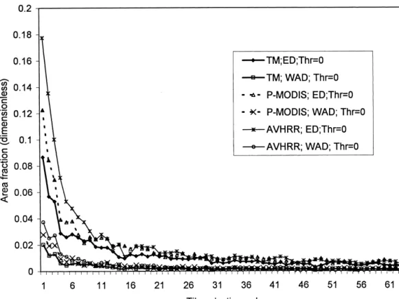
Figure 2 shows the effect of tile selection for three data with approximately 100 Landsat scenes, the latter being
sets (TM, P-MODIS, AVHRR) using Thr50. Two
mea-interpreted visually in the process. As a cross-check on
sures express the difference between whole area and the the AVHRR- map it may be noted that in comparison to
selected tiles, ED [Eq. (1)] and WAD [Eq. (5)]. In all
the independently obtained TM map, the average
abso-cases, the difference diminishes rapidly at first and then
lute difference [DAB, Eq. (6)] for the domain was 0.03%
very gradually until most tiles are selected. The
differ-and the relative difference [DRE, Eq. (7)] 1.6%.
ence became quite small after about 1/6 (for WAD) to
Computation of f and CI 1/3 (ED) of the tiles were selected, depending on data set and measure. It was smallest for the TM set and
The TM-derived map (960035504, 30 m pixels) was
di-vided into 64 tiles (Fig. 7), each consisting of 12003 largest for the AVHRR. This is likely because the small
scale variability was retained in case of TM, thus improv-688 pixels. Secondly, the TM classification was
trans-formed into an equivalent coarser classification by as- ing the representation of class proportions at the tile
level. For AVHRR, the local variability was reduced, and
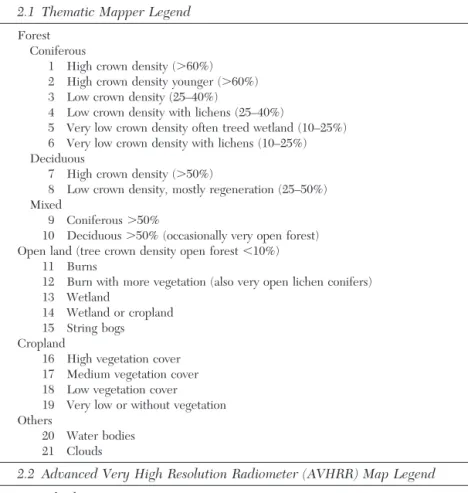
pix-Table 2. Land Cover Types for the Landsat TM and AVHRR Classifications
2.1 Thematic Mapper Legend
Forest Coniferous
1 High crown density (.60%) 2 High crown density younger (.60%) 3 Low crown density (25–40%)
4 Low crown density with lichens (25–40%)
5 Very low crown density often treed wetland (10–25%) 6 Very low crown density with lichens (10–25%) Deciduous
7 High crown density (.50%)
8 Low crown density, mostly regeneration (25–50%) Mixed
9 Coniferous.50%
10 Deciduous.50% (occasionally very open forest) Open land (tree crown density open forest,10%)
11 Burns
12 Burn with more vegetation (also very open lichen conifers) 13 Wetland
14 Wetland or cropland 15 String bogs Cropland
16 High vegetation cover 17 Medium vegetation cover 18 Low vegetation cover 19 Very low or without vegetation Others
20 Water bodies 21 Clouds
2.2 Advanced Very High Resolution Radiometer (AVHRR) Map Legend
Forest land
Evergreen needleleaf forest
1 High density Medium density 2 Southern forest 3 Northern forest Low density 4 Southern forest Deciduous broadleaf forest
5 Northern forest
6 Deciduous broadleaf forest Mixed forest
7 Mixed needleleaf forest
Mixed intermediate forest:
8 Mixed intermediate uniform forest 9 Mixed intermediate heterogeneous forest 10 Mixed broadleaf forest
Burns
11 Low green vegetation cover 12 Green vegetation cover Open land
13 Transition treed shrubland
14 Wetland/shrubland (medium density) 15 Grassland Developed land Cropland 16 High biomass 17 Medium biomass Mosaic land 18 Cropland-Woodland 19 Cropland-Other Other 20 Water
Figure 2. The mean Euclidean distance (ED) and the mean weighted absolute difference (WAD) between the domain and the tiles selected using thresholdThr50.
the tile consisted of fewer pixels, thus requiring addi- which together can strongly contribute to the domain are
selected, the selection becomes so broad as to be effec-tional tiles to obtain a broader, more representative
sam-ple. The P-MODIS result was intermediate between the tively random. The selection is then more strongly
influ-enced by CI. For lower Thr (0.5), the selection is
re-two. The rate of convergence of the sample to the
do-main would thus depend on the relationship between the stricted to a narrower range of tiles, and therefore the
point at which the influence of CI begins to dominate
landscape heterogeneity and pixel size, and secondly on
the size of the tile relative to that of the domain. Figure arrives later. This trend is the same for TM and for
P-MODIS, and also holds for WAD. For the AVHRR
2 also shows that the trends ofEDandWADwere
simi-lar, although ED had a wider range. This is because a (Fig. 3c), ED values for intermediate threshold values
(0.3, 0.5) were also between the Thr50 and random
large difference in a few classes will affectEDmore than
WAD.Thus, ED is a more appropriate criterion for the cases throughout most of the selection process. The
trend shown in Figures 3a and 3b was present as well selection of tiles because it leads to a faster convergence
of the sample to the domain. The advantage of ED is (initial ED decrease followed by an increase), but it
never reached the random case. On the other hand, obvious in some cases, for example, the third selection
step (Fig. 2) for whichEDdecreased strongly (signifying Thr51.0 produced the same ED as the random case. It
suggests that if the spatial distribution of cover types is
fast convergence to domain values) but WAD increased
somewhat. also important (as described byCI), a larger number of
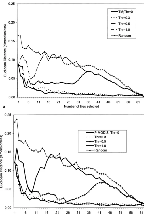
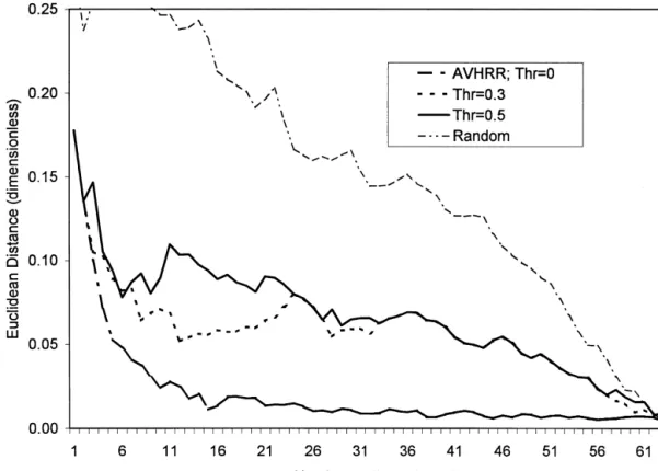
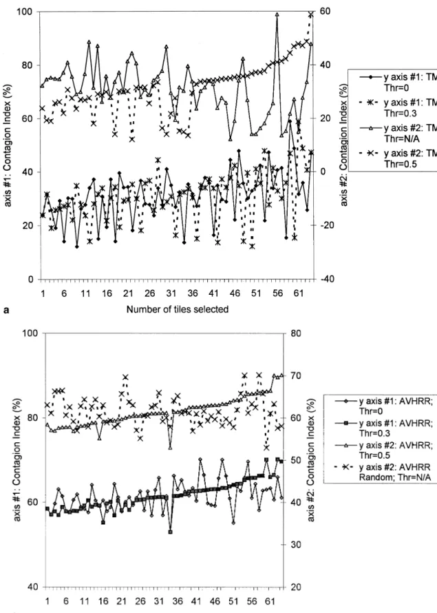
scenes will be required to represent a domain. Figure 3 illustrates the effect of adding the
conta-gion index as a selection criterion. The overall tendency A further insight into the effect of CI on the
selec-tion can be obtained from Figure 4 which showsCI
val-is to approximate the random selection result (top curve,
Fig. 3a). For both the TM (Fig. 3a) and P-MODIS (Fig. ues for individual selected tiles. The CI values for the
domain were 21.5 (TM) and 57.1 (AVHRR). There is a 3b) data sets, the difference between the selections with
Thr50 (i.e., noCIused) andThr50.3 was small and not general trend to increasing CI values starting from the
domain value and the selection based on ED only
systematic. At higher Thr values, ED initially followed
theThr50 curve but then move towards the random se- (Thr50). In other words, the tiles with the highest
diver-sity of cover types (and thereby lowestCI) were selected
lection case. The point at which it starts to deviate
de-pends onThr.At high Thr (1.0), the selection considers first, and subsequent scenes tended to be more
homoge-nous. Second, for lowThrtheCI values of adjacent tiles
Figure 3. The mean Euclidean distance (ED) between the domain and the tiles selected using various
Figure 3. Continued
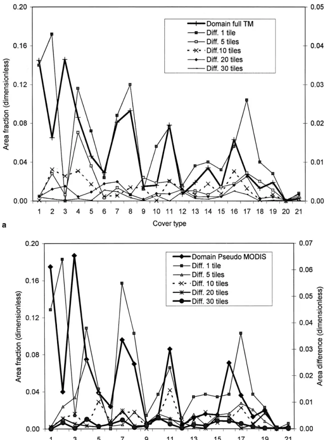
fluctuated substantially but this fluctuation was damp- 5a), it varied between 0% (class 3) and 97% (class 17:
true fraction 2.7%, estimated 0.1%). This was reflected
ened as theThrvalue increased. For higherThr, the CI
values of selected tiles increased almost monotonically in the average errors for all classes, both absolute [DAB,
1.5%, Eq. (6)] and relative [DRE, 41.2%, Eq. (7)].
once the heterogeneous tiles were used up. Thus, the
se-lection was guided by CI once the initial heterogeneous Increasing the number of tiles dampened the
fluctu-ation, leading to average DAB (DRE) errors of 0.3%
scenes were exhausted. In effect, theRCvalues [Eq. (4)]
would differ less between the remaining tiles, thus per- (10%) for 10 tiles and 0.2% (10%) for 20 tiles (i.e., 31%
of the area). Although further reductions were obtained, mitting a larger number of tiles to become candidates for
selection (Step 7). The same trend was observed for TM they were relatively small. For example, by increasing
the number of tiles by 50% (to 30), the average absolute (Fig. 4a) and AVHRR (Fig. 4b). The main difference was
the earlier start of the monotonic increase for AVHRR, error decreased by only 0.1% and the relative error by
4.1%. It should be noted that the relative error was
throughout the Thr50.3 as opposed to a second half of
Thr50.5 selection (TM). The TM curves also show that strongly influenced by two small classes, representing
0.7% and 0.3% of the area, respectively. Without these
the monotonic increase was stronger for higherThr
val-ues. Figure 4 thus implies that theED trends in Figure classes,DREwas 7.6% (10 tiles), 5.9% (20), and 2.6% (30).
A similar trend was observed for the P-MODIS data 3 result from the combined effect of cover type
hetero-geneity (in the candidate tiles) and theThrvalue. When (Fig. 5b). From the high average values after one tile
(DAB52.0%;DRE562.7%), the magnitude decreased to
the former is low and the latter high, the ED curve for
the selected tiles will approximate random case and CI 0.2% absolute and 12.3% (9.2% without two small
classes) relative after 20 tiles. The addition of the next will increase monotonically for adjacent tiles. This trend
is due in part to the way CI is used in the algorithm 10 tiles reduced the errors by 0% and 5.1% (2.0%
with-out the two classes), respectively. The actual AVHRR (Step 8), and is discussed further below.
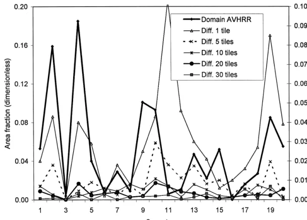
Figure 5 shows the effect of increasing sample size data behaved in a similar way, although the fluctuations
were larger. After one tile, the DAB (DRE) was 3.1%
on the difference between the domain and selected tiles
within the same data set, both on individual classes and (155.4%). These were reduced to 0.5% (22.9%) after 10
tiles and to 0.3% (15.2%) after 20. As in the case of
P-the combined effect. A value of Thr50 was used. For
one tile, the relative difference between the actual and MODIS, the addition of further tiles decreased
ap-preciably only DRE (to 8.8%) while absolute error
Figure 4. The contagion index (CI) between the domain and the tile selected at each step for various threshold values: TM land cover map (a), AVHRR map (b).
Figure 5. The cover type area fraction and the absolute difference between the fraction of land cover type in the domain map and the sample (right-hand y-axis), for individual cover types: TM (a), P-MODIS (b), AVHRR (c). The difference is computed between the domain values for that date type and the sample.
Figure 5. Continued
changed by 0.1%. This is because of three small classes Third, a comparison of Figures 6b and 6c shows that the
small classes magnified the overall relative error. For P-(0.6–0.9% of the area); without these, the DRE values
were 10.2% (with 10 tiles), 8.0% (20), and 4.8% (30). MODIS, the relative error was reduced by 30% when
leaving out the smallest class; for AVHRR, the reduction The trends observed in Figure 5 suggest that the tile
se-lection scheme is less efficient if small classes are present was 20%. Fourth, when TM was used as a reference, the
difference in the DREvalues between tiles selected
us-and must also be well represented, unless they are
spa-tially associated with larger, more ubiquitous classes. ing AVHRR or TM was small: 14.5% (for 10 tiles), 0.9%
(20), and 0.1% (30). Similarly, the difference in relative Since the TM map completely covered the area of
interest it is possible to accurately evaluate the extent to errors was also small for P-MODIS (0.5% for 10 tiles,
1.5% for 20, 0.1% for 30). This shows that full coverage which a sample of the AVHRR tiles would represent the
area if it were imaged at high resolution, that is, the fea- by coarse or medium resolution data can be successfully
used to select representative areas to derive statistics that sibility of using coarse resolution coverage to select a
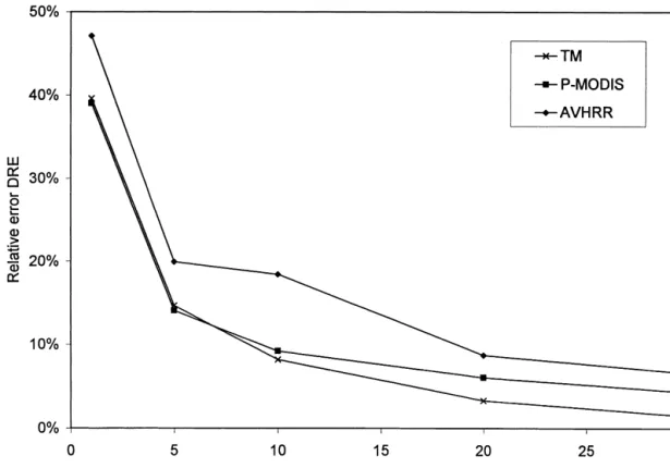
high resolution sample. Figure 6 shows DRE values for are nearly as accurate as if the sample were selected
from full coverage of high resolution data. Although the three data types and different reference data
(Thr50): domain coverage by the same data type (Fig. there is an implied requirement for accurate coarse
reso-lution map, it is more important that the cover classes be 6a); domain coverage by TM (Fig. 6b); and domain
cov-erage by TM but ignoring the smallest class (represent- internally consistent, that is, each coarse resolution class
should be comprised of a reasonably stable fractions of
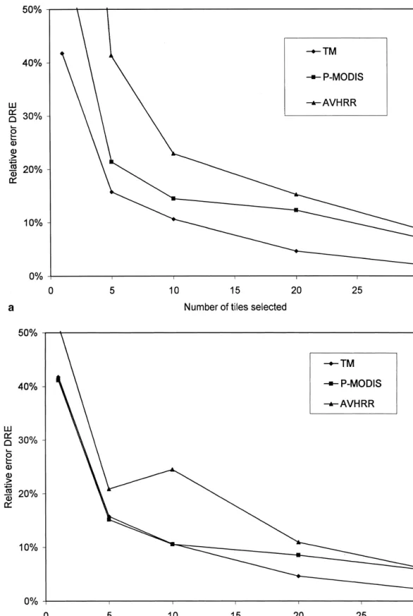
ing 0.3% of the area) in DRE computation. Several
ob-servations can be made. First, the relative error individual classes (that are resolved at high resolution).
Although comparable results after 20 or so tiles can decreased first rapidly and then more gradually, as also
noted in Figure 5. Only in one case (AVHRR, 10 tiles) be obtained, this does not mean that exactly the same
tiles will be selected. Figure 7 shows the tiles selected
did a partial increase (Fig. 6b) occur. Second, theDRE
values for coarser resolution tiles were smaller when from the three data sets. Using the TM data set as a
reference, only seven identical tiles (35%) were selected compared to 30 m pixels (Fig. 6b) than to the same
reso-lution (Fig. 6a), by about 30% for 20 tiles and both from the P-MODIS data set and 11 (55%) from the
AVHRR data. On the other hand, the first five tiles were AVHRR and P-MODIS. At the higher resolution, the
in-dividual classes appear to be represented more accu- chosen in the same order for TM and P-MODIS while
the entire selection sequence was different between the rately because the small classes were not averaged out.
Figure 6. The mean relative error (DRE) between the domain and the selected tiles with different ref-erence data. a) Compared to the domain map of the same data type; b) compared to the TM domain map; c) compared to the TM domain map and without the smallest class (occupying 0.3% of the domain).
Figure 6. Continued
AVHRR and the TM. A full correspondence is not to be area. In this article, representativeness was considered in
expected because small differences in ED may lead to terms of the cover type composition, as expressed by the
different selection paths. Once a different tile is selected, fractions occupied by each class and by the spatial
distri-it affects the subsequent sequence because those tiles bution measured by the contagion index. Using cover
are selected to balance the ones already chosen. The fractions only, the tiles selected with 480 m or 1000 m
similarity of the relative errors after a number of tiles resolution maps provided virtually the same statistics as
were selected (Fig. 6) means that various combinations tiles selected with 30 m data once approximately 1/4 to
of tiles can provide similar results. 1/3 of the area was selected. The number of tiles
in-How closely do the statistics for the selected tile ap- cluded in the coverage would depend somewhat on the
proximate the domain, and are they unbiased? Figure 8 importance of small classes. If the representation of such
shows the mean difference per class between the domain classes is not critical, a smaller number of tiles can be
(TM map) and the sample with sign considered, com- used. After a certain point, more tiles makes only a small
puted as in the Eq. (6) without the absolute values. For contribution to the cover type composition, as evidenced
Thr50, the curves rapidly converged to 0%, especially by the increase from 20 to 30 tiles (31–47% of the area)
for TM and P-MODIS. The convergence was more grad- which decreased the residual errors only marginally.
Fig-ual for AVHRR, but even there the mean difference was ure 2 indicates that the difference between the sample
only 0.0017% after 20 tiles were selected. The difference
and domain statistics was appreciably reduced further from 0 (and thus the bias) is therefore negligible, even
only when almost all tiles were selected. without taking into consideration other sources of error
When using CI as a selection criterion, the process
(such as classification accuracy) in the domain data sets.
becomes more complicated because of the combinations
For Thr50.5, the curve behaved more erratically. This
of land cover distribution within individual tiles. The al-is because the importance of the contagion index
in-gorithm performed as expected, that is, it selected, as far creases at some stage of the selection process (refer also
as possible, scenes with CI similar to the domain. The
to Fig. 3). Neither convergence nor zero bias can
there-problem is that CI’s for most individual tiles will be
fore be assured in this case.
higher than those for the domain because of the reduced complexity of land cover distribution over a smaller area.
COMMENTS The complexity increases as the number of selected tiles
grows. Thus the way theCIwas applied here is not
opti-The above results show the practical feasibility of
consid-Figure 7. Tiles selected after 20 steps using TM map (a), P-MODIS (b), and AVHRR (c).
Figure 8. Mean difference (sign considered) between the fraction of the area occupied by a class in the domain and the sample. The reference used is the TM domain map, except for the AVHRR/ AVHRR curve where the reference is the AVHRR domain map.
ered (Step 8). The preferred approach would be to com- can be made. First, the PSA procedure is designed to
produce an unbiased sample (as compared to the domain
pute a combined CI for all tiles already selected, and
then compute the change in the sampleCI if each indi- of the same data type). Second, the sample will also be
unbiased if a close relationship exists between the
do-vidual tile were added–similarly as forEDin Step 5.
Un-fortunately, this presents a formidable computational de- main maps at coarse and fine resolutions. This is likely
to be the case for larger areas, simple landscapes, large mand, especially for areas of appreciable size. It would
also require some simplification, that is, the selected tiles parcels of individual cover types, or a combination of
these. Third, the “worst case” situation will be infrequent would have to be assumed to constitute a contiguous map,
thus incurring inaccuracies at the seams between tiles. cover types occurring in small patches. They should be
represented well if their occurrence is correlated with For the study area, the sample selected using the
al-gorithm closely represents the region of interest and the the presence of more frequent cover types, for example,
cutovers cooccurring with contiguous dense forest stands. residual errors are very small. In general, the difference
between the domain and the sample is likely to depend When small, infrequent cover types exist independently
of others, their representation will depend on the spatial on the heterogeneity of the land cover distribution in
re-lation to the pixel size and on the size of the tiles. Con- distribution within the tiles. In this study, the worst case
(smallest class) occupied 0.3% of the area in the TM do-sidering typical data types, the tiles can vary between 60
km (SPOT images) and 185 km (TM full scenes), larger main coverage. The DRE values for this class with 20
(30) tiles were 25.2% (15.1%) for TM, 21.7% (36.7%) for than those used here. Thus the convergence between
do-main and sample statistics is likely to be faster because P-MODIS, and 0% (15.1%) for AVHRR. This shows that
coarse resolution does not necessarily cause underrepre-individual tiles will have a more balanced representation
of cover types; this is especially true if full TM scenes sentation of small classes. It is also important to note that
using random selection does not ensure representative-are being selected. Nevertheless, from a statistical
view-point the exact cover type composition of the domain ness unless independent information about the domain is
available (which implies some form of coarse resolution should not be based on a simple average of the selected
tiles. Simple averaging assumes random sampling so that mapping in the broad sense). Even when such
informa-tion is available there is no assurance that a randomly or the sample units can be considered independent. In our
case, the selection is not random as the goal is to select systematically selected sample contains the small classes.
On the other hand, if the classes are mapped at both the minimum representative subset. Three observations
resolutions PSA ensures that the sample is selected in main and the sample diminished rapidly at first and later only slowly with an increasing sample the most efficient way to represent the entire domain for
a given sample size. size. Depending on the data set, the difference
was small to negligible after 1/6 to 1/3 of the do-When analyzing land cover characteristics, it is
desir-able to obtain measures of statistical confidence. In prin- main was selected.
2. Selection using data with 1000 m pixels (AVHRR) ciple, these can be obtained if the probability of each tile
being selected is known and statistical methods based on was nearly as efficient as with 30 m (TM) or 480
m (resampled TM). The average difference in unequal probability sampling are applied (Cochran,
1963). Stuart (1976) demonstrated that in unequal prob- cover type proportions between the domain
(mapped at 30 m) and the sample of 20 tiles was ability sampling, the selection should be made as nearly
proportional as possible to the values of the variable in 0.0002% (TM), 20.0017% (AVHRR), and
0.0007% (P-MODIS). The differences were also the population. Various methods have been used to
com-bine coarse and fine resolution data for land cover analy- small for lower numbers of selected tiles.
3. When ED andCI are used in combination, the
sis (e.g., Walsh and Burk, 1993; Moody and Woodcock,
1996; Mayaux and Lambin, 1995; 1997; Cihlar et al., selected sample represents a combination of the
1997b; Moody, 1998). These methods should yield more two attributes, and may not converge to the
do-accurate results if the selected high resolution sample main uniformly.
closely represents the domain, and an objective and re- 4. The final number of tiles to be included in the
producible method of selecting such sample is strongly sample is a compromise decision which involves
preferable to a subjective procedure. This topic is ex- the residual differences between the domain and
plored in the companion article. the sample at each selection step as well as
practi-As described, PSA does not provide an objective cut- cal (resource) considerations.
off for the sample size. This is a decision to be made by
It is concluded that the PSA algorithm provides an effi-the analyst depending on effi-the requirements of a
particu-cient way to identify a sample of high resolution data for lar study and the financial and other resources available.
multiresolution studies.
The changes in ED (Fig. 2), CI (Fig. 4), DRE (Fig. 6),
and mean difference (Fig. 8) or DAB with increasing
We wish to acknowledge the helpful comments of two anony-number of tiles provide the foundation for the tradeoff
mous reviewers. decisions.
REFERENCES SUMMARY AND CONCLUSIONS
The increasing availability of coarse and fine resolution Ahern, F. J., Janetos, A. C., and Langham, E. (1998), Global
land cover maps presents a requirement for methods to observation of forest cover: a CEOS’ integrated observing
optimally combine these different sources of information strategy. InProceedings of 27th International Symposium on
for studies of landscape characteristics at various spatial Remote Sensing of Environment, Tromsø, Norway, 8–12
June, pp. 103–105.
scales. In practice, it is readily feasible to produce land
Beaubien, J., Cihlar, J., Simard, G., and Latifovic, R. (1999),
cover maps for large areas at coarse resolution and for
Land cover from multiple Thematic Mapper scenes using
smaller areas at high resolution. The question then arises,
a new enhancement-classification methodology.J. Geophys. where should the high resolution sample be taken?
Res., in press.
In this article, we have developed and tested an
al-Belward, A., Ed. (1996), The IGBP-DIS global 1 km land cover
gorithm for an objective sample selection, concentrating
data set: proposal and implementation plan, IGBP-DIS
on the parts of the domain which provide the most
infor-Working Paper #13, The International
Geosphere–Bio-mation content at the high resolution. PSA seeks to find, sphere Programme, IGBP Data and Information System
Of-at each iterOf-ation, the sample unit (tile) which would fice. Toulouse, France. 61 pp.
make the greatest contribution to closing the gap be- Cihlar, J., and Beaubien, J. (1998), Land cover of Canada 1995
tween the characteristics of the whole domain and those version 1.1, Digital data set documentation, Natural
Re-of the sample. We used two descriptors Re-of land cover sources Canada, Ottawa, Ontario.
composition for the selection, fractional distribution of Cihlar, J., Ly, H., and Xiao, Q. (1996), Land cover classification
with AVHRR multichannel composites in northern
environ-various cover types (measured byED) and interspersion
ments.Remote Sens. Environ. 58:36–51.
(quantified by contagion indexCI). When applied to an
Cihlar, J., Ly, H., Li, Z., Chen, J., Pokrant, H., and Huang, F.
area mapped from both AVHRR (1000 m) and TM (30
(1997a), Multitemporal, multichannel AVHRR data sets for
m) images for a 47,500 km2area in central Saskatchewan,
land biosphere studies: artifacts and corrections. Remote Canada, we found that:
Sens. Environ.60:35–57.
Cihlar, J., Beaubien, J., Xiao, Q., Chen, J., and Li, Z. (1997b),
do-Land cover of the BOREAS Region from AVHRR and tion models based on spatial textures. Remote Sens. Envi-ron. 59:29–43.
Landsat data.Can. J. Remote Sens.23:163–175.
McGarigal, K., and Marks, B. J. (1994), FRAGSTATS, spatial Cochran, W. G. (1963), Sampling Techniques, Wiley, New
analysis program for quantifying landscape structure, version York, 413 pp.
2.0, Forest Science Department, Oregon State University, DeFries, R. S., and Townshend, J. R. G. (1994), NDVI-derived
Corvallis, 67 pp. land classifications at a global scale. Int. J. Remote Sens.
Moody, A. (1998), Using landscape spatial relationships to im-15:3567–3586.
prove estimates of land-cover area from coarse resolution Eidenshink, J. C., and Faundeen, J. L. (1994), The 1 km
remote sensing. Remote Sens. Environ. 64:202–220. AVHRR global land data set: first stages in implementation.
Moody, A., and Woodcock, C. E. (1996), Calibration-based
Int. J. Remote Sens.15:3443–3462.
models for correction of area estimates derived from coarse Graham, R. L., Hunsaker, C. T., O’Neill, R. V., and Jackson,
resolution land-cover data. Remote Sens. Environ. 58: B. (1991), Ecological risk assessment at the regional scale.
225–241.
Ecol. Appl1:196–206.
NASA (1982), LANDSAT-4 World Reference System (WRS)
Gustafson,. E. J., and Parker, G. R. (1994), Relationships
be-User Guide, National Aeronautics and Space Administration, tween landcover proportion and indices of landscape spatial
Goddard Space Flight Center, Greenbelt, MD. pattern.Landscape Ecol.7:101–110.
O’Neill, R. V., Krummel, J. R., Gardner, R. H., et al. (1988), Jennings, M. D. (1995), Gap analysis today: a confluence of
Indices of landscape pattern. Landscape Ecol.1:153–162. biology, ecology, and geography for management of
biologi-Salomonson, V. V. (1988), The moderate resolution imaging cal resources.Wildl. Soc. Bull.23:658–662.
spectrometer (MODIS). IEEE Geosci. Remote Sens.
New-Johnson, G. D., Myers, W. L., Patil, G. P., and Taillie, C.
slett. (Aug.):11–15. (1999), Multiresolution fragmentation profiles for assessing
Sellers, P., Hall, F., Margolis, H., et al. (1995), The Boreal hierarchically structured landscape patterns. Ecol. Model.
Ecosystem–Atmosphere Study (BOREAS): an overview and 116:293–301.
early results from the 1994 field year. Bull. Am. Meteorol.
Li, H., and Reynolds, J. F. (1993), A new contagion index to Soc. 76:1549–1577.
quantify spatial patterns of landscapes. Landscape Ecol. Stuart, A. (1976), Basic Ideas of Scientific Sampling, Griffin’s
8:155–162. Statistical Monographs and Courses 4, Hafner, New York, Loveland, T. R., Merchant, J. W., Ohlen, D. O., and Brown, 106 pp.
J. F. (1991), Development of a land-cover characteristics da- Townshend, J. R. G., Justice, C. O., Skole, D., et al. (1994), tabase for the conterminous U.S.Photogramm. Eng. Remote The 1 km resolution global data set: needs of the Interna-Sens.57:1453–1463. tional Geosphere Biosphere Programme. Int. J. Remote Mayaux, P., and Lambin, E. (1995), Estimation of tropical for- Sens. 15:3417–3441.
est area from coarse spatial resolution data: a two-step cor- Turner, M. G. (1990), Spatial and temporal analysis of land-rection function for proportional errors due to spatial aggre- scape patterns.Landscape Ecol.4:21–30.
gation.Remote Sens. Environ. 53:1–16. Walsh, T. A., and Burk, T. E. (1993), Calibration of satellite Mayaux, P., and Lambin, E. (1997), Tropical forest area mea- classifications of land area. Remote Sens. Environ. 46:
281–290. sured from global land-cover classifications: inverse