Efficient Transmission Line Modeling Sensitivity Analysis Exploiting Rubber Cells

EFFICIENT TRANSMISSION LINE MODELING SENSITIVITY ANALYSIS EXPLOITING RUBBER CELLS

P. A. W. Basl†, M. H. Bakr, andN. K. Nikolova

McMaster University Hamilton, ON, Canada

Abstract—The adjoint variable method is applied for the first time to perform sensitivity analysis with transmission line modelingexploiting rubber cells. Rubber cells allow for the conformal modelingof off-grid boundaries in the transmission line modeling computational domain usingmodified tensor properties. The scatteringmatrix of the rubber cell is analytically dependent on the dimensions of the modeled discontinuities. Usingthis property, an exact adjoint system is derived. The original and adjoint systems supply the necessary field information for the rubber cell based sensitivity calculations. Our technique is illustrated through sensitivity analysis of waveguide filters. The estimated sensitivities are used for fast gradient-based optimization and tolerance analysis.

1. INTRODUCTION

Sensitivity analysis plays an important role in the design of microwave circuits. Duringthe optimization procedure, a gradient-based optimizer drives the electromagnetic (EM) simulator. At every iteration, the optimizer requests both the EM response and its gradient with respect to the different design parameters for the current set of parameter values. The response sensitivities are traditionally calculated by perturbingthe design parameters one at a time and then usingfinite difference approximations at the response level. This requires repeated EM simulations of all perturbed EM structures. This process can be time intensive even for a small number of parameters.

The adjoint variable method (AVM) presents a more efficient approach to sensitivity analysis of high frequency structures. AVM † _{The first author is now with CIRFE (Center for Integrated RF Engineering), University}

was utilized with different numerical EM techniques includingthe Method of Moments [1], the frequency-domain Transmission Line Modeling(TLM) [2], the Finite Difference Time Domain (FDTD) with unstructured grids [3], and the Beam Propagation Method in photonics [4]. In [5], the AVM technique was used for sensitivity analysis usingFDTD with structured grids and for full wave sensitivity analysis of guided wave structures [6]. In [7], it was applied to 2D time-domain TLM problems with structured grids involving non-dispersive boundaries and perfect conductingobjects. In all these approaches, usingonly two full wave EM simulations, the sensitivities of a real objective function, with respect to all design parameters, are estimated regardless of the number of these parameters. This represents significant computational saving as compared to the finite difference approximations.

AVM for time-domain TLM was then developed and extended to handle a variety of practical EM design problems. In [8], and [9], the AVM was adapted to handle problems with dispersive boundaries using the wideband Johns matrix boundaries and the one-way wave-equation absorbingboundaries, respectively. The AVM was also extended to solve a variety of EM structures involvingdielectric discontinuities [10], lossy media [11] and full 3D problems [12] usingJohns symmetrical condensed node [13]. The approach was further developed for complex responses to calculate network parameters sensitivities e.g. S-parameters [14]. Self-adjoint S-parameters sensitivities were then introduced in [15] for lossless isotropic homogenous media. The self-adjoint technique uses only the original simulation to calculate the sensitivities over a wide frequency band. No adjoint simulations are needed in this case. The original simulations supply both the S-parameters and their sensitivities with respect to all the design parameters over the desired frequency band. In [16], the adjoint-free AVM was applied to lossless isotropic nonhomogenous media as well.

condensed node [17] and the multigrid TLM [18]. These techniques accurately model on-grid geometries only. Other efforts to model off-grid objects and boundaries include modifying the scattering matrix of the symmetric condensed node [19], loadingit with extra reactive elements [20], and addingextra stubs and/or arms to the boundary TLM nodes [21]. Recently, Huilian et al. introduced in [22] a simple robust approach to model boundaries at arbitrary locations in the TLM symmetric condensed node scheme. This approach depends on modifyingthe constitutive parameters of the irregular boundary cells. This modification accounts for the irregular boundary positions without changing the cell dimensions. Hence, the computational burden remains low.

In [23], we exploited this recent development. We proposed an AVM approach that exploits the rubber cell concept. Usingthe modified tensor properties of these cells, we are able to derive an exact adjoint system for both metallic and dielectric discontinuities. Both types of discontinuities are treated in the same way. Utilizingexact adjoint systems improves the accuracy of the algorithm and makes the implementation process easier for any type of discontinuity. In this paper, we further discuss the proposed approach, explainingits implementation and illustrate it with more examples.

We start by giving a brief review of the use of the modified tensor properties to model irregular boundaries in TLM. In Section 3, we develop the necessary modifications in AVM to perform sensitivity analysis of such structures. Section IV discusses the implementational details of the AVM technique exploitingthe rubber cell. Section 5 illustrates the efficiency of our algorithm through three examples of different microwave filters. Finally, Section 6 shows how the adjoint sensitivities are used to efficiently optimize a microwave filter and perform tolerance analysis without simulatingany perturbed structures.

2. TLM USING RUBBER CELLS

In TLM, both space and time are discretized. The computational domain is modeled through a network of interconnecting transmission lines. The symmetric condensed node is the most common TLM node used for full 3D analysis [13]. Usingthe symmetric condensed node, all boundaries can only be placed half-way between nodes. Global or local mesh refinements can be used to model arbitrarily shaped boundaries. However, this usually leads to increased computational requirements.

representing the changes in the dimensions of a TLM cell through an equivalent change of the cell’s constitutive parameters. The scattering matrix of a TLM cell of size ∆x×∆y×∆zand with material properties characterized by the diagonal permittivity and permeability tensors

←→_{ε =}

εxx 0 0

0 εyy 0

0 0 εzz ; ←→µ =

µxx 0 0

0 µyy 0

0 0 µzz

(1)

is determined using the general formula given in [22]. For the TLM cell shown in Fig. 1 with scaled dimensionsu∆x×v∆y×w∆z, we modify the tensor permittivities and permeabilities associated with the cell to account for the effect of the size change while preserving its original dimensions.

Figure 1. A TLM cell stretched by factors u,v, and w.

The new tensor permittivities and permeabilities are calculated as follows [22]:

ε_xx= vw

u εxx, ε

yy =

uw

v εyy, ε

zz =

uv wεzz µ_xx= vw

u µxx, µ

yy =

uw

v µyy, µ

zz =

uv wµzz

(2)

where u, v, and w are the scalingcoefficients in the x, y, and z directions, respectively. After the new tensors are calculated for each deformed cell, the overall scatteringmatrix is calculated usingthe general formulae in [22].

Utilizingthe rubber cell approach, the TLM simulation carries out a sequence of scatteringand connection steps. The complete TLM step for nondispersive boundaries is given by

where Vk is the vector of incident impulses for all nodes at the kth

time step. S andC are the global scattering and connection matrices, respectively. The vector V_ks is the vector of source excitation at the kth time step.

3. AVM THEORY

Followingthe discussion in Section 2, we conclude that any off-grid discontinuity, whether it is a perfectly conductive obstacle or a dielectric insert, can be modeled by an on-grid discontinuity surrounded by rubber cells with modified tensors. Accordingly, a slight perturbation of a discontinuity results in a perturbation in the surroundingcells tensors. This directly leads to an explicit perturbation in the nodal scatteringmatrix of those cells. Hence, the perturbation can be modeled as an analytical perturbation in the overall scatteringmatrix in a way similar to the case of perturbinga dielectric discontinuity [10].

To calculate the sensitivity of a real objective function F with respect to a design parameter xi, we follow the derivation presented

in [10]. We make use of the analytical derivative of the system matrix A with respect to the tensor properties of the perturbed TLM cells surroundingthe discontinuity. The sensitivity is calculatingusingthe sensitivity expression [10]

∂F ∂xi ≈

∂e_F

∂xi −

∆t

Nt

k=0

λT_k ∂A ∂xi

Vk, i= 1,2, . . . , n (4)

where Nt is the total number of simulation time steps and λk is the

vector of adjoint impulses. λk is calculated usingthe exact adjoint

system [10]:

λk₋1 =STCTλk−V_ks, λ (5)

where V_ks, λ is the vector of adjoint excitation calculated duringthe original simulation.

To calculate the derivative of the system matrix with respect to the design parameter of interest, we consider a case of a general 3D perturbation. For such a perturbation, it is possible that a cell is perturbed in any of the three directions. Usingthe chain rule:

Then usingthe chain rule again we have: ∂A

∂u = ∂A ∂ε_xx ·

∂ε_xx ∂u +

∂A ∂ε_yy ·

∂ε_yy ∂u +

∂A ∂ε_zz ·

∂ε_zz ∂u

+ ∂A ∂µ_xx ·

∂µ_xx ∂u +

∂A ∂µ_yy ·

∂µ_yy ∂u +

∂A ∂µ_zz ·

∂µ_zz ∂u

∂A ∂v =

∂A ∂ε_xx ·

∂ε_xx ∂v +

∂A ∂ε_yy ·

∂ε_yy ∂v +

∂A ∂ε_zz ·

∂ε_zz ∂v

+ ∂A ∂µ_xx ·

∂µ_xx ∂v +

∂A ∂µ_yy ·

∂µ_yy ∂v +

∂A ∂µ_zz ·

∂µ_zz ∂v

∂A ∂w =

∂A ∂ε_xx ·

∂ε_xx ∂w +

∂A ∂ε_yy ·

∂ε_yy ∂w +

∂A ∂ε_zz ·

∂ε_zz ∂w

+ ∂A ∂µ_xx ·

∂µ_xx ∂w +

∂A ∂µ_yy ·

∂µ_yy ∂w +

∂A ∂µ_zz ·

∂µ_zz ∂w

(7)

Since the matrix A is an analytical function of the tensors, its derivatives with respect to the tensors can be analytically calculated. Using(2), (6), and (7), the analytic derivatives ofAwith respect toxi,

i= 1,2, . . . , n, are calculated. They are then used in the sensitivity expressions (4).

There are many advantages of this technique. First is the ability to model any discontinuity without the need to snap it to the grid. Second, the use of analytical derivatives of the system matrices to model the perturbations increases the algorithm accuracy and simplifies the implementation.

Finally no mappingapproximation [8] is needed and an exact adjoint system is used for both metallic and dielectric discontinuities. 4. IMPLEMENTATION DETAILS

In [12], the implementation process of the AVM technique in 3D problems usingthe symmetric condensed node was explained. Figs. 2 and 3 show the nodes affected and the links to be stored when perturbinga perfectly conductingand a dielectric discontinuity, respectively.

(a) (b)

(c) (d)

Figure 2. A perturbation of a perfectly conductingdiscontinuity: (a) impulses stored in original system (top view), (b) impulses stored in original system (side view), (c) impulses stored in exact perturbed adjoint system, and (d) impulses stored in approximate unperturbed adjoint system [12].

a perturbation of the scatteringmatrix of the surroundingnodes. In the rubber cell, the perturbation of a design parameter of either a metallic or a dielectric discontinuity perturbs the nodal scattering matrix of the nodes affected by this particular design parameter. The implementation details are explained in more detail in this section for both types of discontinuities.

4.1. Metallic Discontinuities

(a) (b)

(c) (d)

Figure 3. A perturbation of a dielectric discontinuity: (a) impulses stored in original system, (b) impulses stored in exact perturbed adjoint system, (c) impulses stored in approximate unperturbed adjoint system, and (d) impulses stored in exact unperturbed adjoint system [12] (each group of similar arrows represent impulses to be stored for a particular node).

in Fig. 4(b). The stretching and shrinkage factors of the rubber cells are also shown. The sensitivity expression (4) requires storingvoltage impulses in both the original and adjoint simulations. In the original simulation, we store the impulses reflected from the nodes whose scatteringmatrices are affected by the perturbation of the particular discontinuity.

1-u1 u1

x z

(a) (b)

(d) (c)

Figure 4. Rubber cell implementation for a metallic discontinuity; (a) the off-grid discontinuity, (b) the snapped to grid discontinuity showing the sizingfactors of the rubber cells, (c) the nodes to be stored due to a perturbation in the positivex direction, and (d) the nodes to be stored due to a perturbation in the positivez direction.

4.2. Dielectric Discontinuities

need to be replaced by rubber cells as well. This is the main difference between this case and that of metallic discontinuities. Fig. 5(a) shows an off-grid 2D dielectric object and Fig. 5(b) shows how it is modeled usingrubber cells. Rubber cells are marked with dots in their centers. When the dielectric object is perturbed in a certain direction, the scalingfactors of both the external and internal boundary nodes are

w

1

w

2

1-w

1

1-w

2

1-u1 u1

x z

1-u1 u1

x z

(a) (b)

(d) (c)

changed. Accordingly, we need to store impulses reflected for these two types of nodes. Figs. 5(c) and 5(d) show the nodes affected by perturbation in the positive x- and z-directions, respectively. Accordingly, we store the incident voltages on those cells in the original simulation and their respective reflected impulses in the adjoint simulation.

5. EXAMPLES

The examples presented in this section are simulated usingour in-house TLM simulator coded in Matlab [24]. AVM sensitivities are compared to central finite difference sensitivities calculated at the response level. The response of interest is the absolute value of theS-parameters. Our algorithm provides sensitivities of the real and imaginary parts of the S-parameters. Accordingly, we can also calculate the sensitivities of the magnitude and phase of theS-parameters. The sensitivities of the magnitude are obtained using the formula:

∂|Spq| ∂xi

=

Re{Spq}

∂Re_{Spq} ∂xi

+ Im{Spq}

∂Im_{Spq} ∂xi

|Spq| (8)

wherep and q represent the ports number;p, q= 1,2, . . . , N. 5.1. Three-Resonator Waveguide Filter [15]

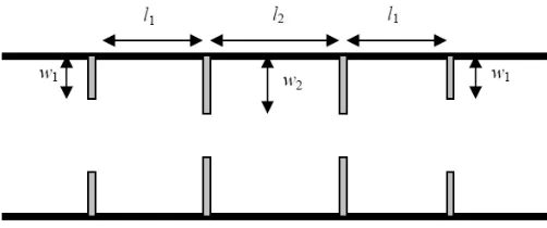
The filter is shown in Fig. 6. The waveguide width is a = 60.0 mm and its length is 180.0 mm. The cell size is ∆l = 1.5 mm. Johns matrix boundaries are used to model the dispersive waveguide ports. Symmetry is used to simulate only half of the structure.

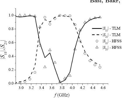
Figure 7. Return and insertion losses for the three-resonator waveguide filter.

The design parameters are the iris widths w1 and w2, and the

resonator lengths l1 and l2. The nominal values are [w1 w2 l1 l2]T =

[14.0 17.0 40.0 45.0]Tmm and the irises have zero thickness. Fig. 7 shows theS-parameters calculated usingour in-house TLM simulator employingthe rubber cell implementation in comparison with the S-parameters calculated using HFSS [25].Very good agreement is obtained between the two simulators. Fig. 8 shows the S-parameters sensitivities calculated with respect to all the design parameters. Good agreement is obtained at most frequencies except at frequencies where the response is highly nonlinear. Using central-difference calculations at the response level requires 8 additional simulations. UsingAVM only 2 full simulations are required. AVM simulations required 473 seconds for the original system, 491 seconds for the adjoint system, and 289 seconds for the postprocessingcalculations of the sensitivities. The total is 1253 for 4 parameters and 29 frequencies. On the other hand usingHFSS and central differences required a total of 9×172 = 1548 seconds for .1in TLM lies in the use of the rubber cell that requires usinga smaller time step to ensure stability.

5.2. Dielectric Resonator Filter [11]

Figure 8. Return loss and insertion loss sensitivities for the three-resonator waveguide filter; |S11| sensitivities calculated using

central-differences (—); |S11| sensitivities calculated usingAVM (◦); |S21| sensitivities calculated usingcentral-differences (- -); and |S21|

sensitivities calculated usingAVM ().

dielectric permittivity is εr = 4.0. The S-parameter sensitivities

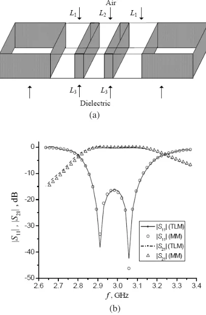
are estimated over a range of frequencies where only the dominant mode is propagating. The sensitivities are calculated at [w d s]T = [18.86 11.32 37.0]Tmm and compared to central-difference sensitivities in Fig. 10. Central-difference calculations require 6 extra simulations, while AVM calculations require only one extra TLM simulation. 5.3. An Evanescent Mode Waveguide Filter [26]

Figure 9. The dielectric resonator filter.

Figure 10. Return loss and insertion loss sensitivities for the dielectric resonator filter; |S11| sensitivities calculated usingcentral-differences

(—); |S11| sensitivities calculated usingAVM (◦); |S21| sensitivities

calculated usingcentral-differences (- -); and |S21| sensitivities

calculated usingAVM ().

tolerances compared to metallic iris waveguides.

The waveguide width is 40.0 mm. The dielectric used has εr =

2.54. The cell size is 1.0 mm. The structure is symmetrical with respect to its 2 ports. The lengths of the air sections arel1 = 13.0 mm

and l2 = 23.0 mm. The two dielectric sections are of equal lengths

l3 = 23.0 mm. The filter is designed and optimized using the mode

(a)

(b)

Figure 11. Evanescent mode waveguide filter: (a) 3-D layout and, (b) the reflection and insertion loss (MM: mode matching).

6. APPLICATIONS OF AVM

In the previous sections we showed how the AVM offers an efficient approach for sensitivity analysis in EM numerical simulations. In this section we present how the AVM sensitivities can be directly used to significantly improve the efficiency of EM design optimization and tolerance analysis.

6.1. Gradient Based Optimization

Figure 12. Return loss and insertion loss sensitivities for the evanescent mode filter; |S11| sensitivities calculated

usingcentral-differences (—); |S11| sensitivities calculated usingAVM (◦); |S21|

sensitivities calculated usingcentral-differences (- -); and |S21|

optimization variables. The design specifications for this filter are:

|S11| ≥0.9 for 2.8 GHz≤f ≤3.27 GHz |S11| ≤0.15 for 3.46 GHz≤f ≤3.95 GHz. |S11| ≥0.9 for 4.34 GHz≤f ≤5.34 GHz

(9)

The initial values of the design parameters are [w1 w2 l1 l2]T =

[14.0 17.0 40.0 45.0]T mm. The filter response for these values is shown in Fig. 13 together with the design requirements. Optimization is done usingthe Matlab [23] minimax optimization algorithm. Gradients calculated usingthe AVM are provided at every optimization iteration. The optimizer reached the optimal set of parameters after 6 iterations usingonly 14 function evaluations includingthose needed for the line search performed per iteration. This means 6 AVM simulations in addition to 8 function evaluations for line search. This is equivalent to a total of 20 TLM simulations. If finite-difference approximations were used, we would need 5 functions evaluations per iteration in addition to the 8 function evaluations for line search resultingin a total of 38 EM simulations.

Figure 13. S-parameters for the three-resonator filter showingthe required design specifications.

It is clear that AVM achieves almost 50% computational savings in the whole optimization process. These savings will be more significant for a problem with larger number of design variables. The optimal values for the design parameters are [w1 w2 l1 l2]T =

Figure 14. The optimized filter response.

Figure 15. The tolerance analysis curves for the three-resonators filter.

6.2. Tolerance Analysis

Since AVM provides response gradients in an efficient way, we used them to predict the response of the optimal design with small tolerances. UsingTaylor’s expansion, the response of the slightly perturbed design can be predicted to be

|S11(x+ ∆x)|=|S11(x)|+

∂|S11|

∂x

T

·∆x (10)

where ∆xlies within the manufacturingtolerance of the process used. Equation (10) is calculated hundreds of times usingrandomly chosen values for ∆x to predict the response of the optimal design when affected by the tolerances. This means only one full wave AVM simulation is needed to perform a complete tolerance analysis. Fig. 15 shows tolerance analysis for the optimized three-resonator waveguide filter example. The tolerance used is 10%.

7. CONCLUSION

The AVM is applied for the first time to TLM problems with conformal boundary modeling. This conformal modelingis achieved usingTLM rubber cells with modified tensors to model irregular cells. Using this novel technique, all perturbations can be modeled as analytical perturbations of the global scattering matrix. The availability of the analytical derivative of the system matrix with respect to any design parameter enables us to derive an exact adjoint system, thus increasing the algorithm accuracy, while simplifying its implementation. We utilized the AVM sensitivities to illustrate efficient gradient-based optimization and tolerance analysis.

REFERENCES

1. Georgieva, N. K., S. Glavic, M. H. Bakr, and J. W. Bandler, “Feasible adjoint sensitivity technique for EM design optimiza-tion,”IEEE MTT-S Int. Microwave Symp. Dig., Vol. 1, 299–302, Jun. 2003.

2. Bakr, M. H. and N. K. Georgieva, “An adjoint variable method for frequency domain TLM problems with conductingboundaries,” IEEE Microwave & Wireless Comp. Letters, Vol. 13, 408–410, Nov. 2003.

4. Swillam, M. A., M. H. Bakr, and X. Li, “Efficient adjoint sensitivity analysis exploitingthe FD-BPM,” J. Lightwave Technology, Vol. 25, 1861–1869, Jul. 2007.

5. Shen, G., H. W. W. Tam, N. K. Nikolova, and M. H. Bakr, “Adjoint sensitivity technique for FDTD methods on structured grids,” IEEE Int. Symp. Antennas & Propagation, 746–749, Columbus, OH, 2003.

6. Swillam, M. A., M. H. Bakr, and X. Li, “Full wave sebsitivity analysis of guided wave structures usingFDTD,” J. Electromagnetics Waves and Applications, Vol. 22, No. 16, 2135– 2145, 2008.

7. Bakr, M. H. and N. K. Nikolova, “An adjoint variable method for time-domain transmission-line modelingwith fixed structured grids,” IEEE Trans. Microwave Theory and Tech., Vol. 52, 554– 559, Feb. 2004.

8. Bakr, M. H. and N. K. Nikolova, “An adjoint variable method for time domain TLM with wideband Johns matrix boundaries,” IEEE Trans. Microwave Theory and Tech., Vol. 52, 678–685, Feb. 2004.

9. Basl, P. A. W., M. H. Bakr, and N. K. Nikolova, “Time-domain sensitivity analysis of planar structures usingfirst-order one-way wave equation boundaries,”Int. Journal. of Numerical Modelling: Electronic Networks, Devices and Fields, to be published.

10. Basl, P. A. W., M. H. Bakr, and N. K. Nikolova, “Efficient estimation of sensitivities in TLM with dielectric discontinuities,”

IEEE Microwave & Wireless Comp. Letters, Vol. 15, 89–91,

Feb. 2005.

11. Basl, P. A. W., M. H. Bakr, and N. K. Nikolova, “Efficient sensitivity analysis of lossy discontinuities usingtime-domain TLM,”Antem/URSI 2006 Conference Proc., 613–616, Jul. 2006. 12. Basl, P. A. W., M. H. Bakr, and N. K. Nikolova, “An AVM

technique for 3-D TLM with symmetric condensed nodes,” IEEE Microwave&Wireless Comp. Letters, Vol. 15, 618–620, Oct. 2005. 13. Johns, P. B., “Symmetrical condensed node for the TLM method,” IEEE Trans. Microwave Theory and Tech., Vol. 35, 370–377, Feb. 1987.

14. Bakr, M. H. and N. K. Nikolova, “Efficient estimation of adjointvariableS-parameter sensitivities with time domain TLM,”

Int. Journal of Numerical Modelling: Electronic Networks,

Devices and Fields, Vol. 18, No. 2, 171–187, Mar. 2005.

“Self-adjoint S-parameter sensitivities for lossless homogeneous TLM problems,” Int. Journal of Numerical Modelling: Electronic Networks, Devices and Fields, Vol. 18, 441–455, Nov. 2005. 16. Basl, P. A. W., M. H. Bakr, and N. K. Nikolova, “Theory of

selfadjoint S-parameter sensitivities for lossless nonhomogeneous transmission-line modelingproblems,” IET Proc. Microwaves, Antennas & Propagation, to be published.

17. Scaramuzza, R. A. and A. J. Lowery, “Hybrid symmetrical condensed node for the TLM method,” Electronics Letters, Vol. 26, 1947–1949, Nov. 1990.

18. Herring, J. L. and C. Christopoulos, “Multigrid transmission-line modelingmethod for solvingelectromagnetic field problems,” Electronics Letters, Vol. 27, 1794–1795, Sep. 1991.

19. German, F. G., “Infinitesimally adjustable boundaries in symmet-rical condensed node TLM simulation,”Applied Electromagnetics Symp. Dig., 482–490, Monterey, CA, 1993.

20. Muller, U., A. Beyer, and W. J. R. Hoefer, “Movingboundaries in 2-D and 3-D TLM simulations realized by recursive formulas,” IEEE Trans. Microwave Thoery and Tech., Vol. 40, 2267–2271, Dec. 1992.

21. Gwarek, W. K., “Analysis of an arbitrarily-shaped planar circuit a time-domain approach,” IEEE Trans. Microwave Thoery and Tech., Vol. 33, 1067–1072, Oct. 1985.

22. Huilian, D., S. Poman, and W. J. R. Hoefer, “Cells with tensor properties for conformal TLM boundary modeling,” 2006 IEEE MTT-S Int. Microwave Symp., Vol. 11, 157–160, San Francisco, CA, USA, 2006.

23. Basl, P. A. W., M. H. Bakr, and N. K. Nikolova, “Efficient transmission line modelingsensitivity analysis exploitingrubber cells,”IEEE MTT-S Conference Proc., 53–56, June 2008.

24. Mathworks, Matlab, “R2007,” ed., 2007. www.mathworks.com 25. Ansoft Corporation, “HFSS,” 9.2.1 ed., 2004. www.ansoft.com 26. Beneat, J., “Design of high frequency filters for data transmission

& evanescent mode waveguide structures,” PhD thesis, Univ. de Bordeux, 1993.