Application of Taguchi Grey Relational Analysis to optimize the process
parameters in wire electrical discharge machine.
Mr.Vinit Raut1, Mrs. Meeta Gandhi 2 Mr Nilesh Nagare3 Mr. Aniket Deshmukh4
1
Mechanical Department, D.J.Sanghvi College of Engineering Vile Parle (E), Maharashtra, India
2
Mechanical Departments, , D.J.Sanghvi College of Engineering Vile Parle (E), Maharashtra, India
3
Mechanical Department, VIVA Institute of Technology, Virar (E), Maharashtra, India
4
Mechanical Department, VIVA Institute of Technology, Virar (E), Maharashtra, India
Abstract
In this report the effect of Process parameters on material removal rate(MRR) and surface roughness of HCHCR-D2(high carbon high chromium steel) die steel are investigated as MRR and Surface roughness in W-EDM(wire electrical discharge machining) are of crucial importance and Taguchi L9 orthogonal array and Grey Relational Analysis techniques are used for optimization of parameters. For experimentation Pulse on time (Ton), Pulse off time (Toff), Peak current (Ip), and wire feed rate(Wf) are taken as input parameters while MRR and Surface roughness are taken as output parameters. For each experiment Surafce roughness is calculated by using Surface finish tester and MRR is calculated by measuring the difference in weight of workpiece before and after machining with time required for machining.
Keywords: Wire electrical discharge machining,
HCHCR-D2 Material, Taguchi Grey Relational analysis technique..
1.
Introduction
1.1 Wire Electrical Discharge Machining Process:
Wire Electrical Discharge Machining (W-EDM) is widely used manufacturing process used to machine conductive materials due to its capability of producing intricate and complex shapes irrespective of hardness and toughness of material. It can produce more complex two and three dimensional shapes through conducting materials This process is extensively used in mould and die making industries, nuclear industry, aerospace industry etc. . In
WEDM (wire electrical discharge machining) material removal takes place due to electro thermal process. A series of electrical pulses generated by pulse generator unit is applied between the work piece and travelling wire electrode which generate series of discrete sparks between the electrode and work piece. While the machining is continued, the machining zone is continuously flushed with water passing through the nozzles on both sides of the work piece.
2. Problem Definition:
In CNC Wire electrical discharge machine, Process parameters like pulse on time(Ton), pulse off time(Toff), Input Current(Ip), wire feed rate(Wf) play an important role as it affects the MRR (material removal rate) and Surface roughness. Most of the times this machines are operated by workers; If process parameters are not set properly then it results in low MRR as well as Surface finish. If at some point amount of stock removed from the electrode becomes greater than the amount being removed from the work piece, the wire electrode breaks and discharge is stopped.The overall objective is to produce
high quality product at low cost to the
manufacturer.Optimization is a process that finds a best, or optimal, solution for a problem of process parameters is the best way to solve this problem. Taguchi L9 Orthogonal array and Grey Relational analysis used to set optimal set of parameters.
3. Methodology:
3.1 Design of Experiment:
The design of experiments (or experimental design) is the design of any task that aims to describe or explain the variation of information under conditions that are hypothesized to reflect the variation. The term is generally associated with true experiments in which the design introduces conditions that directly affect the variation, but may also refer to the design of quasi-experiments, in which natural conditions that influence the variation are selected for observation.
3.2 Work piece Material:
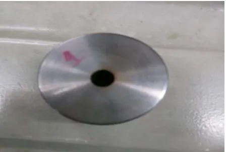
The work piece material is HCHCR-D2 (high carbon high chromium steel) with dimension (Diameter 40mm, Thickness 26mm, weight 230gm) is used for experimentation. The Brass wire with diameter 0.25mm is used as electrode. Pure distilled water is used as dielectric medium. Fig. 4.2 shows actual working zone of WEDM and Table 4.1 shows the Percentage of Composition of HCHCR-D2.
Table 3.1: Percentage of Composition of HCHCR-D2 (Wt %)
C Mn Cr Si
2 0.2-0.35 12 0.2-0.35
Fig.3.1: Work piece
Fig.3.2: Working zone of Wire electrical discharge machining
3.3 ELECTRA Wire Cut Electric Discharge Machine:
ELECTRA Wire Cut Electric Discharge Machine
(Manufactured by Electronica Machines Tools Ltd) is used
in this investigation. Once wire is wound on the wire drum,
that particular amount of wire is used for all experiments
of each material and it has been replaced once the material
is changed. Work material is tightly clamped on working
table with the help of suitable fixture so as to avoid any
Constant dielectric flow is ensured during the
experimentation.Fig.3 shows the CNC WEDM machine
used for experimentation.
Fig 3.3: Wire-EDM Machine
4. Case Study:
In experimental study 8mm hole is created in the work
piece with brass wire. MRR (material removal rate) is
calculated by measuring the difference in weight of work
piece before and after machining and time required to
create a through hole. Surface roughness (Ra) is calculated
by MITUTOYO Surface Tester Master.
4.1 Taguchi L9 Orthogonal Array:
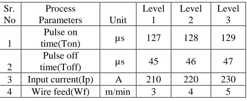
Table 5.1 shows process parameters with their level for
this experiment. The Taguchi method involves reducing
the variation in a process through robust design of
experiments. The overall objective of the method is to
produce high quality product at low cost to the
manufacturer.
Table 4.1: Process parameters with their levels.
Sr. No
Process
Parameters Unit
Level 1
Level 2
Level 3
1
Pulse on
time(Ton) µs 127 128 129
2
Pulse off
time(Toff) µs 45 46 47
3 Input current(Ip) A 210 220 230
Taguchi Proposed to acquire the characteristics data by
using orthogonal arrays, and to analyse the performance
measure from data to decide the optimal process
parameters. The designed matrix of input parameters with
output parameters such as MRR (material removal rate)
and Surface roughness (Ra) for HCHCR-D2 (High carbon
high chromium steel) shown in table 5.4. Selection of a
particular OA is based on the number of levels of various
factors. Here, Number of levels (L)=3 and No of
factors(f)=4 therefore Degree of Freedom (DOF) can be
calculated by using Eq. as DOF = f x (L-1) =8,the
orthogonal array should be equal to or greater than
DOF,here 9>8 hence L9. Each machining parameter is
assigned to a column of OA and 9 machining parameter
combinations are designed.
Table 4.2: Designed matrix of input and output parameters
Trial
No Ton Toff Ip Wf
MRR
(gm/min) Ra(µm)
1 127 45 210 3 0.66 1.9
2 127 46 220 4 0.92 2.1
3 127 47 230 5 1 2.7
4 128 45 220 5 0.66 1.8
5 128 46 230 3 1.06 1.9
6 128 47 210 4 0.82 1.3
7 129 45 230 4 1.12 1.4
8 129 46 210 5 0.82 1.8
9 129 47 220 3 1.12 1.5
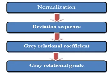
4.2 Grey relational Analysis:
The grey analysis was first proposed many decades ago but
has been extensively applied only on the last decade. Grey
analysis has been broadly applied in optimizing the
The multi-objective problem can be converted into single
objective optimization using GRA technique.
Fig. 4.1: purpose of grey relational analysis
In Grey relational analysis, experimental data i.e.,
measured features of quality characteristics are first
normalized ranging from zero to one. This process is
known as Grey relational generation. Next, based on
normalized experimental data, Grey relational coefficient
is calculated to represent the correlation between the
desired and actual experimental data. Then overall Grey
relational grade is determined by averaging the Grey
relational coefficient corresponding to selected responses.
The overall performance characteristic of the multiple
response process depends on the calculated Grey relational
grade. This approach converts a multiple response process
optimization problem into a single response optimization
situation with the objective function is higher Grey
relational grade. The optimal parametric combination is
then evaluated which would result highest Grey relational
grade.
4.2.1 Steps in GRA
Fig. 4.2: Steps in GRA
(a)Normalization:
It is the first step in the grey relational analysis; a
normalization of the S/N ratio is performed to prepare raw
data for the analysis where the original sequence is
transferred to a comparable sequence. Linear
normalization is usually required since the range and unit
in one data sequence may differ from the others. A linear
normalization of the S/N ratio in the range between zero
and unity is also called as the grey relational generation.
Further analysis is carried out based on these S/N ratio
values. When the range of the series is too large or the
optimal value of a quality characteristic is too enormous, it
will cause the influence of some factors to be ignored. The
original experimental data must be normalized to eliminate
such effect. There are three different types of data
normalization according to whether we require the LB
(lower-the-better), the HB (higher-the-better) and NB
(nominal-the-best). The normalization is taken by the
following equations.
…...………
………. (4.1)
(b) LB (lower-the-better)
………...
.……… (4.2)
(c) NB (nominal-the-best)
………
……….……… (4.3)
Here, i= 1, 2… m; k=1, 2… n
Where x i (k) is the value after the grey relational
generation, min y i (k) is the smallest value of y i (k) for
the kthresponse, and max y i(k) is the largest value of y i
(k)for the kthresponse. An ideal sequence is x0(k) for the
responses. The purpose of grey relational grade is to reveal
the degrees of relation between the sequences say, [x0 (k )
and x i (k ) , i = 1, 2,3...,9].
(b)Determination of deviation sequences,
The deviation sequence is the absolute the reference
sequence x0(k) and the comparability sequence xi(k) after
normalization. It is determined using
= |x0 (k) - xi (k)|
……….……… (4.4)
(c) Calculation of grey relational coefficient
(GRC)
GRC for all the sequences expresses the relationship
between the ideal (best) and actual normalized S/N ratio. If
the two sequences agree at all points, then their grey
relational coefficient is 1.
………
……….……… (4.5)
Where, difference of the
absolute value ; is the
distinguishing coefficient 1;
= the
smallest value of ; and =
= largest value
of . Comparability sequence and ζ is the distinguishing
coefficient. The value of can be adjusted with the
systematic actual need and defined in the range between 0
and 1, ∈ [0, 1]. It will be 0.5 generally.
(d)Determination of grey relational grade (GRG):
The overall evaluation of the multiple performance
characteristics is based on the grey relational grade. After
averaging the grey relational coefficients, the grey
relational grade can be computed as:
………
…...……… (4.6)
Where, n = number of process responses.
If the two sequences agree at all points, then their grey
relational grade of two comparing sequences can be
quantified by the mean value of their grey relational
coefficients and the grey relational grade. The grey
relational grade also indicates the degree of influence that
a comparability sequence could exert over the reference
sequence. Therefore, if a particular comparability sequence
is more important than the other comparability sequences
to the reference sequence, then the grey relational grade for
that comparability sequence and reference sequence will be
higher than other grey relational grades.
The higher value of grey relational grade corresponds to
intense relational degree between the reference sequence
x0(k) and the given sequence xi (k). The reference
sequence x0(k) represents the best process sequence.
Therefore, higher grey relational grade means that the
corresponding parameter combination is closer to the
optimal.
Based on Taguchi’s L9 Orthogonal Array design, the
predicted data provided can be transformed into a
signal-to-noise (S/N) ratio; based on three criteria. The loss
function (L) for objective of HB and LB is defined as
follows:
LHB
= ...
... (4.7)
LLB
= ………
……….(4.8)
Table 4.3 Signal-to-Noise Ratio
Response values S/N Ratio
MRR(gm/min) Ra(µm) MRR(dB) Ra(dB)
0.66 1.9 -3.60912 -5.5751
0.92 2.1 -0.72424 -6.4444
1 2.7 0 -8.6273
0.66 1.8 -3.60912 -5.1055
1.06 1.9 0.506117 -5.5751
0.82 1.3 -1.72372 -2.2789
1.12 1.4 0.98436 -2.9226
0.82 1.8 -1.72372 -5.1055
1.12 1.5 0.98436 -3.5218
Table 4.4: Normalization
Tria l No
S/N Ratio Normalized S/N Ratio
MRR(db) Ra(db) MRR Ra
1 -3.6091 -5.5751 0 0.51921755
2 -0.7242 -6.4444 0.628037292 0.656151699
3 0 -8.6273 0.785704938 1
4 -3.6091 -5.1055 0 0.4452428
5 0.50612 -5.5751 0.895886568 0.51921755
6 -1.7237 -2.2789 0.410450818 0
7 0.98436 -2.9226 1 0.101394498
8 -1.7237 -5.1055 0.410450818 0.4452428
9 0.98436 -3.5218 1 0.195790518
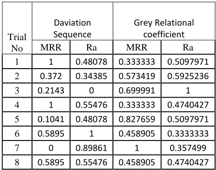
Table 4.5: Deviation sequence and grey relational
coefficient
Trial No
Daviation
Sequence Grey Relational coefficient
MRR Ra MRR Ra
1 1 0.48078 0.333333 0.5097971
2 0.372 0.34385 0.573419 0.5925236
3 0.2143 0 0.699991 1
4 1 0.55476 0.333333 0.4740427
5 0.1041 0.48078 0.827659 0.5097971
6 0.5895 1 0.458905 0.3333333
7 0 0.89861 1 0.357499
9 0 0.80421 1 0.383374
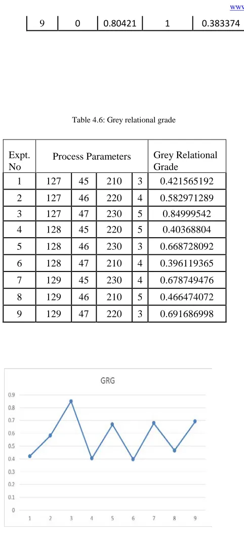
Table 4.6: Grey relational grade
Expt. No
Process Parameters Grey Relational
Grade
1 127 45 210 3 0.421565192
2 127 46 220 4 0.582971289
3 127 47 230 5 0.84999542
4 128 45 220 5 0.40368804
5 128 46 230 3 0.668728092
6 128 47 210 4 0.396119365
7 129 45 230 4 0.678749476
8 129 46 210 5 0.466474072
9 129 47 220 3 0.691686998
Fig. 4.3: Scatter plot of GRG vs order of experiment.
The mean of the grey relational grade for each level of the
machining parameters is summarized and shown in Table
4.7
Table 4.7: The Main Effects of the Factors on the Grey Relational Grade
Level 1 Level 2 Level 3
A Ton 0.6182 0.4895 0.6123 0.1287 3
B Toff 0.5013 0.5727 0.6459 0.1446 2
C Ip 0.5709 0.5594 0.7325 0.1616 1
D Wf 0.594 0.5526 0.5734 0.0414 4
Rank Grey Relational Grade
symbol Paramete r
Main Effect
The larger the grey relational grade, the better is the
multiple performance characteristics. However, the relative
importance among the machining parameters for the
multiple performance characteristics still needs to be
known, so that the optimal combinations of the machining
parameter levels can be determined more accurately.
Table4.7, the optimal parameter combination was
determined as A1(pulse on B3(pulse off
time)-C3(Input current)-D1(wire feed rate).
4.2.2 Confirmation Test:
The purpose of the confirmation experiment is to validate the conclusions drawn during the analysis phase. After determining the optimum level of process parameters, a new experiment is designed and conducted with optimum levels of CNC W-EDM parameters obtained.
Table 4.8: Confirmation results
Predicted Experimental Error
MRR(gm/min 0.99 1.06 0.07
Ra(µm) 2.22 2.26 0.04
These values and percentage error between actual and predicted values of the responses are given in table 4.8 The percentage error between the actual and predicted values of the responses falls below 5%, which shows that the optimized value of CNC W-EDM process parameters obtained is good enough for achieving the target set during the experiment. The comparison again shows the good ,
4. Conclusions
Taguchi’s L9 orthogonal array and Grey relational analysis were applied to improve the multi response
characteristics such as MRR (material removal rate) and
Surface roughness (Ra)
(a)The optimal parameter combination determined as A1(pulse on time)-B3(pulse off time)-C3(Input current)-D1(wire feed rate),Table 5.5
(b)Input Current(Ip) has maximum influence on both MRR and Surface Roughness.
(c) MRR and Surface Roughness increases with increase in Input Current (Ip).
References
[1] Prasenjit Datta and Bikash Choudhary, “Optimization of Wire edm machining in Inconal 800 using Grey relational
analysis”, Proceeding of IRF international conference, pp.17-21,2015.
[2] G.Antony Casmir and S. Ashok kumar, “ Optimization of wire cut edm using hchcr by taguchi analysis”, International conference on recent advancement in mechanical engineering &technology, pp.54-57, 2015.
[3] Timur Rizovich Ablyaz and Vladimir Aleksandrovich Ivanov, “Research of Electrical Discharge Machining Process of Wear Resistance Coatings Obtained By Beam Deposit
Process”,journal of Modern Applied Science, vol 9, pp.257-265, 2015.
[4]Amit Chauhan and Onkar Singh Bhatia, “Optimization of multiple machining characteristic in wedm of nickel based super alloy using of taguchi method and grey relational analysis”, International Journal of Advanced Technology in Engineering and Science, vol.3,pp.187-193 ,2015.
[5]Vijay D Patel and Dr. D M Patel, “A Study and Investigation on SR in Wire Electrical Discharge Machining using
Molybdenum Wire”, International Journal On Innovative Research in Science, Engineering and Technology, vol 3,pp.45-56, 2014.
[6] Brajesh Lodhi and Sanjay Agarwal,“Modeling of Wire Electrical Discharge Machining of AISI D3 Steel using response Surface Methodology”,5th Intrnational manufacturing
technology, Design and Research Conference (AIMTDR 2014) December 12th–14th, IIT
2014.
[7] Anurag Joshi, “Wire cut edm process limitations for tool and die steel”, International Journal of Technical Research and Applications,vol 2,pp. 65-68, 2014.
[8] Richa Garg and Saurabh Mittal, “ Optimization by Genetic Algorithm”, International Journal of Advanced Research in Computer Science and Software Engineering,vol 4, pp. 587-589, 2014.
[9] Shaaz Abulais, “Current Research trends in Electric
Discharge Machining(EDM)”, International Journal of Scientific & Engineering Research, Vol 5,pp. 100-118, June-2014.
[10] K.B.Rai and P.R.Dewan, “Parametric optimization of WEDM using grey relational analysis with Taguchi method”, International journal of research in Engineering and Technology, vol. 2, pp. 110-116, 2014.
[11] Dragan Rodic and Marin Gostimirovic, “Predicting of machining quality in electric discharge machining using intelligent optimization techniques”, International Journal of Recent advances in Mechanical Engineering (IJMECH), Vol.3,pp 1-9, 2014.
[12] V. D. Shinde and Anand S. Shivade, “Parametric
Optimization of Surface Roughness in Wire Electric Discharge Machining (WEDM) using Taguchi Method”, International Journal of Recent Technology and Engineering (IJRTE), vol. 3, pp. 10-15, 2014.