Quantum Dots in Graphene

(1)

Quantum Dots in Graphene

V.A. Fedirko

Moscow State University of Technology “Stankin” (MGTU “Stankin”), Russia National Research University of Electronic Technology “MIET” (MIET), Russia

Abstract

The paper reports on theoretical study of electron states for a quantum dot in a graphene monolayer. Discrete energy spectrum of quasiparticles inside the quantum dot is found. Energy levels and corresponding quasiparticle resonant wave functions are obtained, which allow calculating the local density of states inside the quantum dot. Some experimental results recently released are referred.

Keywords

Graphene, Quantum Dot, Quantum

Tunneling, Quasi-localized States

1. Introduction

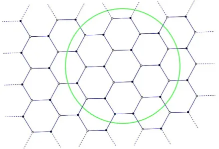
Graphene is a mono-atomic layer of carbon atoms arranged on a 2D honeycomb lattice (Fig 1.). Since the first publication of K.S. Novoselov et al. [1, 2] graphene “has rapidly changed its status from being an unexpected and sometimes unwelcome newcomer to a rising star” [3] and has firmly established itself in condensed matter physics. It is a unique material which has been attracting unfading interest as a fascinating system for fundamental studies and is considered as perspective material for various applications (see, e.g. [3,4]).

Electronic structure of graphene is well described elsewhere (see, e. g. the review article [5]. Near each corner of the hexagonal first Brillouin zone (also called Dirac points or K-points) the quasiparticle excitations obey 2D linear dispersion relation and behave like 2D massless “relativistic” particles, e. g., neutrino. That leads to a number of its unusual peculiar electronic properties [1-5].

Using technological tailoring or electric field a potential relief can be created in a graphene layer which gives new interesting phenomena and provides new opportunities for its application. As was shown in [6] an electron in graphene can, in some states, perfectly pass through the potential barrier independently of its height, just like in quantum electrodynamics – effect well known as Klein paradox [7]. That is in fact a sort of interband tunneling [8-10]: from a valence band state (hole-like) to the conduction band state

(electron-like) in case of a quantum well (QW) or from a conduction band state (hole-like) to the valence band state (electron like) in case of a quantum barrier (QB). However, as was shown in [11] alongside with such delocalized “Klein tunneling states” 1D elementary excitations localized mainly in the quantum well, may exist in a QW of enough power - they form a sort of a peculiar quantum “rod” in a grapheme monolayer. Also conventional valence electron tunneling through a QW may take place in some states [11].

In view of that it is interesting to consider a possibility of localized electron states in a “quantum dot” (QD) in a graphene monolayer. Recently discrete structure of electron density of state was observed in scanning tunneling electron spectroscopy experiment with single-layer graphene [12], which was interpreted just in terms of electron wave resonances in a localized p-n junction formed by field effect. So in this paper we undertake the theoretical study of stationary electron states in a quantum dot in a graphene monolayer.

Underscore that we consider the QD inside formally unbounded graphene layer, not touching upon tunneling out from graphene through its edge [13].

2. Model and Theory

We consider the stationary electron states in a circularly symmetric potential:

0, ( )

0,

U a

V

a ρ ρ

ρ

< < 

=  _>

 , (1)

where ρ is the polar radius, U>0 is the QD depth, a is the QD size, and assume that the states of nonequivalent valleys around opposite Dirac points do not mix (“zigzag” form of the boundary conditions which are the most typical [14,15]). Then we can describe the electron excitations near Dirac points by two-component wave functions

( . ) [ , ]x y _A _B

y = j j obeying 2D Dirac-Weyl–like equation [5,16-18]:

{

0

}

ˆ

(2)

velocity), σ =(σx

,

σ

y) are the Pauli matrices, I is the 2x2 unit

matrix, ∇ = ( /∂ ∂ ∂ ∂x, / y), j j_A, _B being respectively the envelope amplitudes on sublattices A and B of graphene honeycomb lattice (Fig. 1).

Figure 1. A schematic fragment of graphene lattice with a circular quantum dot.

Further we are interested in electron states with the energy 0>E>U and put:

0 , 0 ; 0, 0

E U− =v k E = −vk > >k k .

In view of (1) we thus come to the following set of equations: ( ) ( ) ( ) ( ) B A A B B A A B i ik x y a i ik x y i i x y a i i x y ϕ ϕ ρ ϕ ϕ ϕ kϕ ρ ϕ kϕ ∂ ₋ ∂ ₌  

∂ ∂ _{ <}

 ∂ ₊ ∂ ₌ _  ∂ ∂ _ ∂ ₋ ∂ _{= −}  

∂ ∂ _{ >}

 ∂ ∂ _ + = −  ∂ ∂ _ (3)

Substituting φB from the second equation of each pair into the first one leads to:

2 2 2 2 2 2 2 2 2 2 ( ) ( ) A A A A k a x y a x y

ϕ ϕ ρ

ϕ k ϕ ρ

∂ ∂

+ = − , <

∂ ∂

+ = − , >

∂ ∂

. (4)

Due to the circular symmetry it is convenient to use polar coordinates (ρ,θ); it gives:

2 2

2

2 2 2

2 2

2

2 2 2

( , ) 1 ( , ) 1 ( , ) _{( , )}

A A A

A

A A A

A

k a

a

ϕ ρ θ ϕ ρ θ ϕ ρ θ _{ϕ ρ θ ρ} ρ ρ

ρ ρ θ

ϕ ρ θ ϕ ρ θ ϕ ρ θ _{k ϕ ρ θ ρ} ρ ρ

ρ ρ θ

∂ ₊ ∂ ₊ ∂ ₌ _{, <}

∂

∂ ∂

∂ ₊ ∂ ₊ ∂ ₌ _{, >}

∂

∂ ∂

(5)

We then search for the solution of Eqs. (5) in the form:

( , ) ( ) ( )

A RA A

ϕ ρ θ = ρ Θ θ . Then immediately find:

( ) in A θ e θ n

Θ = , = 0,1, 2...

which leads to the Bessel equation for Z(z)=RA(ρ=z/k) if ρ<a, or Z(z)=RA(ρ=z/κ) when ρ>a:

2 2

( ) 1 _{( ) (1} _{) ( ) 0}

d Z z dZ z _{n Z z}

z dz

dz + + −z = .

We put thus: ( ) (1) (2) ( ) (1) (2) ( ), ( ) ( ) ( ), ( ) , ( ) [ ( ) ( )] , n n n A

n n n n in n n

n

A _in

n n n n

A J k a

R

B H C H a

A J k e a

,

B H C H e a

θ

θ ρ ρ

ρ

kρ kρ ρ

ρ ρ

ϕ ρ θ

kρ kρ ρ

< 

= ⇒

+ <



 ⋅ <

 = 

+ <



, (6)

where Jn(z) is the Bessel function of the order n, Hn(1)(z) and

Hn(2)(z) are the Hankel functions of the order n of the first and the second kind respectively which describe the incident and reflected circular waves, An, Bnand Cn are the constants.

Using the well-known recurrent relation for cylindrical functions [19]: 1 ( ) _{( )} _{( )} n n n dZ z

z nZ z zZ z

dz − = − +

we then find from (3):

( 1) 1

( )

(1) (2) ( 1)

1 1

( )

,

( )

[

( )

( )]

,

i n n n n

B _{i n}

n n n n

A J k e

a

,

B H

C H

e

a

θ

ρ

ϕ ρ θ

kρ

ρ

+ +

+

+ +



⋅

<



= 

+

>



. (7)

For a stationary state in a closed QD the current across its border must be zero. The current density j in graphene is defined by the formula(see, e.g., [14]):

(

)

0

v ψ ψ

=

j s ,

from which we find with (6) and (7) for the current density jρ normal to the circular border of a QD (1):

2 ( )

1

( ) ( )

n

n n n

jρ = A J ka J + ka . (8) That leads for the condition

( ) 0

n

J ka = , (9.1) or

1( ) 0

n

J + ka = , (9.2) which define the discrete energy eigenstates Em in the QD. Evidently it is sufficient to consider Eq. (9.1) only, as (9.2) coincide with the next of (9.1), so

0 0

0, / ,

( / );

nm nm nm nm

nm nm

E U v k k z a

k U v m

k

= + < =

= − + = 1, 2...



 , (10)

[image:2.595.67.287.138.288.2]

(3)

functions will be:

To match the wave function inside and outside of the QD one must put for the states defined by Eq. (9.1):

(1) (2)

1 1 1

( ) ( ) 0

( ) ( ) ( )

nm nm nm nm n nm

nm n nm nn n nm nm n m

B H a C H a

A J k a B H a C H a

k k

+ + +

+ =

= + (11)

That allows finding the ratios Bnm /Anmand Cnm /Anm and thus to determine the wave function outside the QD, Amn considered as normalizing factor:

(2) 1

(1) (2) (1) (2)

1 1

(1) 1

(1) (2) (1) (2)

1 1 ( ) ( ) / ( ) ( ) ( ) ( ) ( ) ( ) / ( ) ( ) ( ) ( )

n nm n nm nm nm

nm n nm n nm nm

n n

n nm n nm nm nm

nm n nm n nm nm

n n

J k a H a

B A

H a H a H a H a

J k a H a

C A

H a H a H a H a

k

k k k k

k

k k k k

+ + + + + + ⋅ = ⋅ − ⋅ ⋅ = − ⋅ − ⋅

. (12)

The corresponding wave functions for Enm energy state inside the QD thus will be:

( )

( ) ( 1)

1

( ) ( / )

( ) ( / ) ,

nm in

nm nm nm A

nm i n

nm n nm B

, A J z a e

, A J z a e a

θ

ϕ ρ θ ρ

ϕ ρ θ ρ + ρ

+

= ⋅

= ⋅ < . (13)

The local electron density in a (nm) state is found as:

2 2

2 ₍ ₎ ₍ ₎

(nm) nm nm

B A

ψ = ϕ +ϕ ; (14)

according to Eqs. 6, 7 it does not depend on polar angle θ. To calculate the density of states inside the QD we normalize the wave functions per unit probability in the QD area:

2 2 2

1 0

1

2 2 2

1 0

2 [ ( ) ( ) ] 1

2 [ ( ) ( ) ]

a

nm n nm n nm

a

nm n nm n nm

A J k J k d

π ρ ρ ρ ρ

+ − + + = ⇒   ⇒ = +     

∫

.(15)

Using the well-known formula for Bessel functions

( )

n

J αz under the condition J_n( ) 0α = [19]:

1 2 2 1 0 1 [ ( ) ( ) 2 n n

J αz zdz= J ₊ α

∫

,

it can be written in the form taking (10) into account: 2 1 2 2 2 1 1 0 1

( ) 2 ( )

nm

n nm n nm

A

a J z J z d

π ₊ ₊ ξ ξ ξ

=   +     

∫



. (15.1)

A good approximation for (14.1) can be obtained from the same formula for Bessel functions:

2

2 2

2

1 2 2 1

1 1

( ) ( )

nm

n nm n n m

n m

A

z

a J z J z

z

π ₊ ₊ ₊

+ ≈   +       (15.2)

which is valid already for n>1 and even for n=0, 1, m≥2. The similar procedure for the states defined by Eq. (9.1) is obvious from Eqs. (6), (7), (9.2). All the (nm) states other than (0m) are thus doubly degenerate. seen from asymptotic of the Bessel functions [19]: their zeros z_nm and z_{n m}_{' '} are very close if

1 _' 1 _'

2 2

m+ n m= + n ,

and get closer with m increasing. For example in a QD with powerful enough potential, say μ=31, five highest levels

010, 29, 48, 67, 86

E E E E E lie in the interval 0

(29.55 30.64)¸ v a/ , i.e. mean interlevel distance 0

0.25( / )

E v a

(4)

[image:4.595.134.477.79.458.2]

Figure 2. Scheme of energy levels in a QD, e =Ea v/ ₀: a - μ=3, b - μ=5, c- μ=6.5, d - μ=6, e - μ=6.8, d- μ=10.5; red – n=0 series, green – n=1, orange – n=2, violet – n=3.

We consider above the QD formed by the negative potential U<0 (1), the quasiparticle stationary states inside the QD are therefore the conduction band, electron-like states. It is quite obvious, that the same approach can be applied for the positive potential U>0 in (1). In that case the quasiparticle stationary states inside the QD will be the valence band, hole-like states.

It is important to note that local electron density in stationary states (10) inside the QD is not uniform. Being independent on the polar angle θ it varies with ρ as follows from (13) and (14) in accordance with the corresponding Bessel functions:

2 ( )

2 2 2

1

( , )

[ ( ) ( ) ]

nm

nm n

n nm n nm n nm

D E g

g A J k J k

ρ η ψ

η ρ ₊ ρ

= =

= + (16)

where g=4 is the spin and valley degeneration factor and ηn is the above mentioned degeneration factor of Enmstate (ηn=1 for n=0, and ηn=2 for n=1, 2, …).

In the center of the QD all the Bessel functions but J0 are

equal to zero, while J0(z) has it maximum value J0(0)=1;

J1(z)<0.6 and has it maximum at z≈2,Jn(z)<0.5 for n>1, and

their first maximum is at z>3. So near the center of the QD only the states of low n series contribute substantially to the electron density. For the example in Fig. 2f only levels E0m

(red lines) and E1m (green lines) are actually essential up to

ρ~0.2a; as seen they are almost equidistant with

ΔE≈1.8(ħv0/a). Say, for a=40nm one has ΔE≈30meV. Most

probably just that was the case observed in [12].

The results though are strictly relevant to the QD with the discontinuous potential (1) will certainly hold qualitatively for more smooth potential too.

3. Conclusions

(5)

quasiparticle states are the conduction band, electron-like ones, while inside the quantum dot formed by the positive potential they are the valence band, hole-like states. Energy levels and corresponding quasiparticle resonant wave functions are obtained, which allow calculating the local density of states inside the quantum dot. Experimental results newly available are briefly referred to from that point of view.

Acknowledgements

The author thanks his daughter Mary Fedirko for help in preparing the illustrations.

The work is supported by the Russian Foundation for Basic Research, Project No. 14-01-00663-a.

REFERENCES

[1] K. S. Novoselov, A. R. Geim. , S. V. Morozov, D. Jiang, Y. Zhang, S. V. Dubonos, I. V. Grigorieva, A. A. Firsov. Electric Field Effect in Atomically Thin Carbon Films, Science, Vol. 306, 666–969, 2004.

[2] K. S. Novoselov, A. K. Geim, S. V. Morozov, D. Jiang, M. I. Katsnelson, I. V. Grigorieva, S. V. Dubonos and A. A. Firsov. Two-dimensional gas of massless Dirac fermions in graphene, Nature,Vol. 438, 197–200, 2005.

[3] A. K. Geim. Graphene: Status and Prospects, Science, Vol. 324, 1530–1534, 2009.

[4] A. K. Geim and K. S. Novoselov. The rise of graphene, Nature Materials, Vol. 6, 183–191, 2007.

[5] A. H. Castro Neto, F. Guinea, N. M. R. Peres, K. S. Novoselov, and A. R. Geim. The electronic properties of grapheme, Rev. Mod. Phys., Vol. 81, 109–162, 2009. [6] M. I. Katsnelson, K. S. Novoselov, and A. R. Geim. Chiral

tunneling and the Klein paradox in graphene, Natur. Phys, Vol. 2, No. 9, 620–625, 2006.

[7] O. Klein. Die Reflexion von Elektronen an einem Potentialsprung nach der relativistischen Dynamik von Dirac, Zeitschrift für Physik, Vol. 53, No. 3-4, 157–165, 1929.

[8] A. G. Aronov and G. E. Pikus. Tunnel Current in a Transverse Magnetic Field, Sov. Phys. JETP, Vol. 24, No. 1, 188–197, 1967.

[9] M.H. Weiler, W. Zawadzki, and B. Lax. Theory of Tunneling, Including Photon-Assisted Tunneling, in Semiconductors in Crossed and Parallel Electric and Magnetic Fields, Phys. Rev. Vol. 163, 733–742 ,1967.

[10] V. A. Fedirko, M.-H. Chen, C.-Ch. Chiu, Sh.-F. Chen, K.-H. Wu, J.-Y. Juang, T.-M. Uen and Yi-Sh. Gou. An explicit model for a quantum channel in 2DEG, Superlattices and Microstructures, Vol. 31, No 5, 207–217, 2002.

[11] V.A. Fedirko. Graphene Electron States in a Quantum Well, UJPA Vol. 9 No. 4, 175–181, 2015, online available from http://www.hrpub.org.

[12] Y. Zhao, J. Wyrick, F.D. Natterer, J. F. Rodriguez-Nieva, C. Lewandowski, K. Watanabe, T. Taniguchi, L.S. Levitov, N.B. Zhitenev, J.A. Stroscio. Creating and probing electron whispering-gallery modes in graphene, Science, Vol. 348 (6235), 672–675, 2015.

[13] C. W. J. Beenakker. Colloquium: Andreev reflection and Klein tunneling in graphene, Rev. Mod. Phys., Vol. 80, No.4, 1337–1354, 2008 (arXiv:0710.3848v2 [cond-mat.mes-hall]). [14] A. R. Akhmerov and C. W. J. Beenakker. Boundary

conditions for Dirac fermions on a terminated honeycomb lattice, arXiv:0710.2723v3 [cond-mat.mes-hall] , 1–10, 2008. [15] V.A.Fedirko. Electron Tunneling from Graphene, UJPA. Vol. 2, No. 6, 263–267, 2014, online available from http://www.hrpub.org

[16] McClure, J. W. Diamagnetism of graphite., Phys. Rev., Vol. 104, 666–671, 1956.

[17] Semenoff, G. W. Condensed-matter simulation of a three-dimensional anomaly, Phys. Rev. Lett., Vol. 53, 2449–2452, 1984.

[18] DiVincenzo, D. P., and E. J. Mele. Self-consistent effective-mass theory for intralayer screening in graphite intercalation compounds, Phys. Rev., Vol. B29, 1685–1694, 1984.