113
A Petri Net Based Approach For Modelling Of
Resource Shared Distributed Wireless Sensor
Networks
Sonal Dahiya, Sunita Kumawat, Priti Singh
Abstract: An extension of Petri net, Dynamic Augmented Marked Petri Net is presented and used for the modeling of systems which can be distributed, dynamic or concurrent in behavior. This paper presents a component based method for modelling an integrated system for multiple distributed wireless sensor networks sharing a common server. Firstly, WSN components are modeled as Dynamic marked petri net and then Dynamic augmented marked petri net is introduced and used for modeling an integrated system where more than one DWSN share a common server. In this technique we have used property preserving composition of Dynamic Augmented Marked Petri Net to a common sharing resource place. The correctness and feasibility of the system designed is verified with the help of property analysis of the system.
Index Terms: Distributed Wireless Sensor Network, Petri Net, Shared Resource, Synthesis and Composition.
—————————— ——————————
1.
INTRODUCTION
Wireless Sensor Networks (WSNs) are prominently used in industrial and scientific societies. These are used in every field of life like transportation and logistics, precision agriculture and animal tracking, environmental monitoring, urban terrain tracking and structure monitoring, entertainment, surveillance and security, health monitoring, smart grid and energy control systems, industrial applications and so on [11]. WSN is a combination of multifunctional and autonomous sensor nodes. These nodes are scattered in a zone to capture an event or to measure a physical magnitude of the event. After capturing the information from the surroundings, these nodes send it to base station which is away from the coverage area. [1], [2]. In Distributed wireless sensor networks (DWSN) [3] each node has the ability to sense, analyze and communicate the information or data from the surroundings. A big number of sensor nodes are required for gathering information about a large area or surrounding in a network. Sensor nodes coordinate among themselves for gathering and processing useful data and communicate the same to base station. Sensor nodes are generally powered by small consumable batteries which cannot be replaced. These nodes should consume very low energy in order to increase lifetime of WSN. So, the main concern in designing the network is to increase lifetime of network which is influenced by protocols selected for WSN. Hierarchical protocols are most efficient in terms of energy which attracts the researchers. Energy constraints are the detriment of other factors, like packet loss which is interesting area of research these days. Hostile nature in WSNs creates errors during routing and it is responsible for packet loss during transmission. To design a reliable WSN, we
must consider significant number of packet losses with efficient power management, especially in critical applications. There, packet loss factor decide performance of a WSN. Simulators are used for analysis of properties and performance evaluation of network protocol designed for WSN. However, a protocol provides good results on simulators but may fail completely in real world. A fault in protocol can reduce lifetime of WSN and can increase packet loss [4]. Petri Nets (1962) are used to design, analyze and evaluate performance of WSN. PN express and represent formalism for modeling discrete event system while events occur after a deterministic time, immediately or after an exponentially distributed time [5]. Not only the network but even the node in a network or processor used in nodes can be easily modeled efficiently by using PN and it outperforms the simulation based and mathematical models [6]. A wireless sensor modeling for evaluation of performance, especially energy consumption with packet loss constraint is widely used. These metrics are used to minimize data packet loss and maximize network lifetime before implementing routing protocols in real world [12].
This paper presents a new extension of Petri net used for the modeling of systems which can be distributed, dynamic or concurrent in behavior. A component based method is used to design an integrated system for multiple Distributed Wireless Sensor Networks sharing a common server. Firstly, the WSN components are modeled as Dynamic Marked Petri Net and then Dynamic Augmented Marked Petri Net is introduced and used for modeling an integrated system where more than one DWSN share a common server. In this approach we used property preserving composition of Augmented Marked Petri Net to a common sharing resource place. The accuracy and feasibility of whole designed system is verified with the help of property analysis of the system.
2
PETRI
NET
AND
PROPERTIES
2.1 Petri Net
A Petri Net (PN) is a weighted, directed, two-part multigraph. It is a graphical and mathematical modeling tool used for defining and analyzing the behavior of a system. Being a graphical tool, it has the capabilities of a flowchart, block ________________________
Sonal Dahiya, PhD Scholar, Amity School of Engineering and Technology, Amity University Haryana, Gurgaon, India. Email: [email protected]
Dr. Sunita Kumavat, Assistant Professor, Amity School of Applied Sciences, Amity University Haryana, Gurgaon, India. Email: [email protected]
114 diagram while being a mathematical tool it is possible to derive
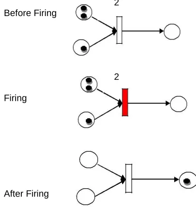
state equations or algebraic equations as required. Petri nets were first introduced for representation of chemical equations in 1962 by Carl Adam Petri in his dissertation [5]. A Petri Net i.e. place/transition net or P/T net consists of places which represent all possible states of a system and transitions which represent actions required to change states, and arcs. Arcs run from either a place to a transition or transition to place and never run from place to place or transition to transition. Input places are the places from which an arc goes to a transition while output places are places to which arc runs from a transition. In the Petri Net representation of a system, circle denotes a place while box or bar denotes a transition also; an arc is denoted by a line with directions. Another significant part of a PN is token. Tokens are allocated to places and are represented by black solid dots and represent change of state with the help of movement from one place to another. Firing of a transition represents occurrence of an event but is dependent upon availability of sufficient tokens at all input places. A transition consumes the tokens from input places equal in number to its associated weights sum of its input arcs and puts the token to the output places equal in number to its associated weights sum of its output arcs. So, tokens initially in places should be grater or equal to its associated output arcs for firing the corresponding output transitions [7]. See Fig. 1 for the process of Petri Net.
2 Before Firing
2
Firing
After Firing
Fig. 1 Petri Net
Definition 1. A Net is a triple N= (P, T, F) where: P and T are disjoint finite sets of places and transitions, respectively. F⊂ (P×T) ∪ (T×P) denotes set of arcs i.e. flow relations, either from place to transition or transition to place.
Definition 2. A place-transition net (PT-Net) is a 5 tuple PN = (P, T, F, W, M0), where,
P is the set of places; T is the set of transitions; such that, P T and P T = ;
F (P T) (T P) is the set of arcs and W: F {1, 2 ...} is the weight function and
M0: P {1, 2, 3…} is initial marking. We ignore unity weight generally in model representation, See Fig. 1for model
description.
In a PN, an initial marking is a function which decides how to distribute tokens to the places initially. Here M0 (p) is a non-negative integer number which is associated with place p and it represents the number of tokens in place p at initial marking M0. M0 (p) is <= to the capacity k of the place p, where capacity of the place is defined as the maximum number of tokens which can be accommodated in place at any reachable marking M from M0. A marking M0 is said to be reachable to M, if there is a firing sequence σ = {t1, t2,…,tn} such that M can be obtained from M0 after firing of transitions t1, t2,…, tn. The execution of Petri nets cannot be determined until we have a predefined execution policy. Multiple transitions can be enabled at same point of time and any one out of them can fire because tokens can be present at more than one place at the same time so, Petri Nets are suitable for modeling concurrent, synchronous, distributed, parallel and even nondeterministic systems [7],[8].
2.2 Properties of Petri Nets
A Petri net is model of a system supports the analysis of properties and difficulties related with discrete event systems. The properties which can be studied with the help of PN model of a system are briefly discussed in this section.
2.2.1 Structural properties
Structural properties of PNs depend only on their topology and are independent of the initial marking. In [5] necessary and sufficient conditions for structural boundedness, conservativeness, repetitiveness and consistency of a PN are provided. A brief overview is presented in this paper.
Boundedness: A Petri Net is said to be k bounded or simply bounded if the number of tokens in each place are not more than k for any marking which is reachable from M0i.e.for initial marking, where k is an integer value. Also, a PN is structurally bounded if it is bounded for any finite initial marking.
Conservativeness: A Petri net PN is conservative if there exists an-vector of positive Integers y ∈Zn y>0 such that for every initial marking M0 and for every marking M which is reachable from M0 the relation MTy = M0Ty=a constant is true.
In case that equality holds for an n-vector of integers y ∈ Z n, y>≠0, then the net is said to be partially conservative.
Repetitiveness: A Petri net PN is called repetitive if there is an initial marking M0 and a firing sequence S such that every transition occurs infinitely often in S. Also, if there is an initial marking M0 and a firing sequence Sin a way, some transitions (not all) occur infinitely often in S, the Net is said to be partially repetitive.
115 firing sequence S from M0 back to M0 such that some
transitions (not all) occur at least once in S.
2.2.2 Behavioral properties
The properties depending upon initial marking are called Behavioral properties.
Reachability: If for a given PN with M0as initial marking and Mr any other marking then, Mr is known as reachable from M0 if and only if there exists a firing sequence which brings the net from M0 to Mr. Thus, reachability set can be defined as the set of all reachable markings fromM0 and is represented by R(M0). It is worth mentioning here that reachability set is defined for a particular initial marking and will change with any change in initial marking.
The dependency implies that reachability is a behavioral property. If Mr is reached from M0 by firing a single transition, then Mr is said to be immediately reachable from M0.
Liveness: Mathematically, a PN is called Live with respect to an initial marking M0 if it is possible to fire all the transitions at least once by some firing sequence where every marking belongs to the reachability set [1].
3
DWSN
COMPONENTS
AS
DYNAMIC
MARKED
PETRI
NET(DMPN)
The modelling of DWSN in form of petri nets can be done in two parts. The first part is to develop model for every component and to know the firing rules while the second part is to combine the components for proper functioning of system. Generally, A PN doesn’t include any specific reference to time, i.e. they are asynchronous in nature. However, it is observed that a few PN extensions may include explicit time delays on either firing of transitions (after being enabled) or token insertion and therefore, token movement and marking vector becomes time dependent. But still, the structure of the PN i.e. places, transitions, and arcs remain time invariant. Dynamic marked Petri net with reference to time has been used to model distributed wireless sensor network. To simplify the DMPN model we assumed that there is a bounded universal set of places and transitions for DMPN. The upper bound on total number of places is Pmax and the upper bound of total number of transitions is Tmax. In DMPN model, we have used three different types of places: PL, PC and BR i.e. location places, channel places and base resource places respectively. Also, two transitions types are TS and TR i.e. sending message transitions and receiving message transitions respectively.
Mathematically,
P = PL PC BR i.e. | PL PC BR | Pmax Where, P is set of all places
PL = {pl1, pl2, pl3, pl4…,pln} where PL is set of location places. PC = {pC1, pC2, pC3, pC4 … ,pCn} where PC is set of channel places.
BR = {r1, r2, r3. . . , rn } where BR is set of base resource places.
Also,
T= TS TR i.e. | TS TR | Tmax where, T is set of all transitions.
TS = {ts1, ts2, ts3, ts4…,tsn} where TS is set of sending message transitions.
and TR = {tr1, tr2, tr3, tr4…,trn} where TR is set of receiving message transitions.
Any place/transition associated with DMPN structure is known as active/alive/enable else that place/transition is known inactive/dead/disable. Also, transitions or places can change the states from active to inactive and vice-versa.
Dynamic Marked Petri Net (DMPN):
For modeling the DWSN, we start with the definition of Dynamic Marked Petri Net i.e. DMPN = [P, T, F, M0 (p) t], where M0(p)t = {M0(p1)t, M0(p2)t,…, M0(pn)t} is initial marking vector at time delay t assigning tokens to the places where M0 (pi)t represents the number of tokens in Pi place at M0.
The initial marking at t time delay, defined as
M0 (pi) t = 0 when pi PL 1 when pi PC BR
After firing of transitions new tokens are assigned to all places and therefore, their marking will be changed. The firing rules are defined as:
Transition tsi belongs to TS is enabled if pLi pRi = 1, i.e. minimum one token available in pLi and pRi both.
Transition tri belongs to TR will be enabled only if pCi
(pLi+1 pRi) = 1.
Now the modelling of the components of a simple Distributed Wireless Sensor Network is presented in Fig. 2.
Modeling of DWSN components:
PN model of location place PL is drawn in Fig. 2(A). It has two inputs and one of the inputs is the outcome of firing of itself, whereas other inputs are the outcome of the shortest channel places. A channel place denotes virtual channel existing between the two nodes for the purpose of communication and we have assumed that every location place will send information to those location places only, which lies within the shortest channel distance and therefore consumes less power. Thus, the channel place as shown in Fig. 2(B) has one input and one output. TS is represented as shown in Fig. 2(C). It receives a message from a location place and transmits this message through single or multiple channel places to base resource location place or/and through other location places. As TR receives a token from its previous channel place it will start firing and sends a token to the next location place after a time delay t (Fig. 2(D)). We can conclude that the location place will not consume token.
116 (C)
(D)
Fig. 2 Petri Net structure of components of a DWSN
4 DYNAMIC
AUGMENTED
MARKED
PETRI
NET
A Dynamic Augmented Marked Petri Net has a delay time t, on insertion of tokens in different places. Mathematically, Dynamic Augmented Marked Petri Net is (DMPN, M0 (p)t; R) is a PT-net (DMPN, M0 (p)t) with a subset of R Places, Resource Places, i.e.:
Every Place in R is marked by M0.
A Dynamic Marked Petri Net graph ( D M P N ' , M0' (p) t) is obtained from (DMPN, M0(p)t; R) after eliminating the places in R and associated arcs.
For every place P belonging to R, there is k > 1 pair of transitions Dk = { (ts1, tr1), (ts2, tr2),..., (tsk, trk)} i . e . r* = { ts1, ts2,..., tsk} T S a n d *r = {tr1,tr2,..., trk } T R a n d that, for each (tsi, tri) Dk, there exists an elementary path in connecting tsi to tri.
In (DMPN', M0' (p)t), every cycle is marked, an example of DMPN is shown in Fig.3.
Fig.3 Dynamic Augmented Marked Petri Net Graph
Composite Dynamic Augmented Marked Petri nets:
Let (DMPN1, M0 1( p ) t ; R 1 ) a n d ( D M P N 2, M0 2( p ) t ; R 2) a r e t w o D y n a m i c Augmented Marked Petri Nets, in which R1' = { r11, r12 r13,. . . , r1k } R1 and R2' = {r21, r22 , r23..., r2k} R2 are the common resource places. Let r11 and r21 be fused as one single place r1, r12 and r22 into r2, a n d s o o n . Here result net will be a Dynamic Augmented Marked Petri Net (DMPN, M0( p ) t ; R ) a n d i s k n o w n a s composite dynamic augmented marked Petri net.
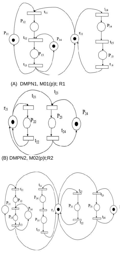
F i g . 4 ( A ) a n d F i g . 4 ( B ) represent the two Dynamic Augmented Marked Petri Nets (DMPN1, M0 1( p ) t ; R1) a n d ( D M P N 2, M0 2( p ) t ; R 2) w h i l e Fig.4 represents the composite d y n a m i c Augmented Marked Petri Net (DMPN, M0( p ) t ; R ) .
(A) DMPN1, M01(p)t; R1
(B) DMPN2, M02(p)t;R2
Fig. 4 Composite model of (A) & (B)
5 INTEGRATED
SYSTEM
OF
DISTRIBUTED
WIRELESS
SENSOR
117 tsi. Sensor location places send information through
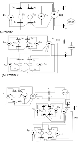
transmitting transition and channel places to base location places and then to the server. Therefore, an integrated network of more than one base station which share common server is attained which the help of composition of two DMPN-structures model of BS1and BS2 to common server. Fig. 5
(A) DWSN1
(A) DWSN 2
Fig. 5 Integrated System of DWSN1 & DWSN2 sharing common server
6
PROPERTY
ANALYSIS
OF
INTEGRATED
SYSTEM
OF
DWSN
PN toolbox in MATLAB can be used to model and investigate a large number of systems modeled by PN. The Petri Net Toolbox (PN Toolbox) is a software tool for simulation, analysis and design of discrete event systems, based on Petri net (PN) models. This software is inserted as a toolbox in the MATLAB environment and to use it MATLAB version 6.1 or higher is
required. Although there are many software tools like Great SPN, J Petri Net, Petri.NET Simulator, QPME etc. for analysis and simulation of PN models [9] but PN Toolbox has its own efficacies. PN toolbox can operate with infinite-capacity places, since MATLAB has the built-in function Inf, which returns the IEEE arithmetic representation for positive infinity whereas in other PN software, places are meant for having finite capacity (as the arithmetic representation used by the computational environment). The integration of MATLAB and PN Toolbox has broadened the utilization domain [10].
The PN Model for above network can be constructed using PN Toolbox in MATLAB as shown below in Fig. 6.
Fig. 6 PN Model for Integrated system of DWSN shown in Fig. 5
The incidence matrix for further mathematical analyses can be calculated as shown below in Fig. 7.
118 The model is found to be live that means each transition is
fired at least once and therefore, each state is significant in this model, as shown in Fig. 8.
Fig. 8 Liveness of Model
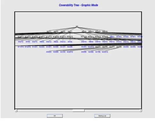
The cover-ability tree explaining the movement from one state to another can be made in graphic mode using PN Toolbox as shown in Fig. 9.
Fig. 9 Cover-ability Tree for model
As can be seen below in Fig. 10 and 11 the model is not only conservative but also consistent i.e no tokens are consumed during the process.
Fig. 10 Conservativeness of Model
Fig. 11 Consistency of Model
7
CONCLUSION
The Petri net has applications in almost all areas of engineering and science especially communication models. In last decade, the Petri net theory is used very frequently in technical scenarios because of its efficacy in analysis of various systems. Through this paper, we presented an expansion of Petri Nets to Dynamic Augmented Petri Net, which is utilized to model system behavior with some structural changes in general PN models. In this paper modeling and property analysis of integrated system of Wireless Sensor Networks sharing common server is represented and standard properties like boundedness, liveness, conservativeness, repetitiveness and consistency are studied which shows that system model is working and there is no deadlock conditions. The cover-ability tree has been drawn and incidence matrix has also formulated for further analysis of the system behavior.
REFERENCES
[1] Catello Di Martino, “Resiliency assessment of wireless sensor networks: a holistic approach” PhD Thesis, Federico II, University of Naples, Itly, December 2009. [2] Bashir Yahya, Jalel Ben-Othman, Lynda Mokdad, and
Seringe Diagne, “Performance evaluation of a medium access control protocol for woreless sensor networks using Petri Nets”, In HET-NET’s2010, pp.335-354, 2010. [3] Ian F Akyidiz, Weilian Su, Yogesh Sankarasubramaniam and Erdal Cayirci, “Wireless Sensor Networks: A Survey”, Computer Networks vol. 38, Iss.4, pp. 392-422, 2002. [4] Jackson Francomme, Karen Godary and Theirry Val,
“Validation formelle d’un mechanism de synchrinisation pour reseaux sans fil”, CFIP’2009, October 2009.
[5] T. Murata, “Petri Nets: Properties, Analysis and Applications”, Proc. Of the IEEE, vol.77, pp541-580, 1982. [6] Ali Shareef and Yifeng Zhu, “Effective Stochastic modelling of energy constrained wireless sensor networks”, Journal Computer Network and Communication, 2012.
[7] Sunita Kumawat, “Weighted Directed Graph: A Petri Net based method of extraction of closed weighted directed Euler trail” International Journal of Services, Economics and management, vol. 4, Iss. 3, pp252-264, ISSN: 1753-0830, 2013.
[8] Victor Khomenko, Olivier H Roux, “Application and theory of Petri Net and Concurrency” Proc. Of 39thInernational conference, PETRI NETS 2018, Bratislava, Slovakia, June 24-29, 2018
119 [10] K.H. Mortensen, Petri Nets Tools and Software,
http://www.daimi.au.dk/PetriNets/tools, 2003.
[11] Bushra Rashid, Mubashir Husain Rehman, “Applications of wireless sensor networks for Urban areas: A Survey”, Journal of Network and computer Applications, vol. 60, 192-219, 2016.