Feature Extraction and Clustering of Twenty Three IIPs of India

268

Feature Extraction and Clustering of Twenty Three IIPs

of India

Dipankar Das1, Nabanita Mukherjee2, Rayna Roy3, Tatini Dasmal4

Department of BCA1,2,3,4,The Heritage Academy, Kolkata, West Bengal, India1,2,3,4 Email: [email protected]2

Abstract-The study analyzes the ‘Index of Industrial Production’ of twenty three (23) different items of India by

extracting the trend, spike, curvature, linearity and entropy features of each of the twenty three (23) indexes. The authors also cluster this time series data on the basis of five (5) extracted features. The largest clusters of indexes were exhibited by both the linearity and spike features. For each of them i.e. linearity and spike features, the larger cluster contains nineteen (19) indexes. Outlier clusters were also identified in the cases of trend, linearity, spike and curvature features. The cluster analysis of the indexes together on spike and linearity gave us a single cluster with twenty (20) indexes while three (3) indexes were marked as outlier cluster.

Index Terms-Feature extraction; Clustering; Time Series; IIP.

1. INTRODUCTION

A time series carries profound importance in business and policy planning, is a sequence of well defined numerical data given in a consecutive order over a period of time (with equal time intervals) [21] mainly have (i) seasonal, (ii) trend, (iii) cyclical and (iv) random variations [22]. Trends [23], Seasonal cycles [24], Non seasonal cycles [25], Pulses and steps [26] and Outliers [27] are the key features of a time series. Feature extraction is used to solve the problem related to time series [28].

Clustering is the task of grouping a set of similar objects which have common attribute or features to each other in a particular group. This technique has many applications [29] in various fields e.g. market segmentation, social network analysis, anomaly detection. Different types of clustering algorithms are available e.g. K Means Clustering [31], Two Step Clustering [32], Hierarchical Clustering [33].

The ‘Index of Industrial Production’ (IIP) of India is an important economic indicator. “The all India IIP is a composite indicator that measures the short-term changes in the volume of production of a basket of industrial products during a given period with respect to that in a chosen base period” [30][36]. Uncovering knowledge of this time series data through an in-depth analysis and data mining is a challenging work.

In the present work, the authors had analyzed the twenty three (23) IIPs of India. In the initial phase, the features of these time series data were extracted and in the last phase the IIPs were clustered using the extracted features.

2. LITERATURE REVIEW

To address the problems in spatial effects of sensory data in time series, Pan, Lin and Gui (2019) developed a “singular value decomposition (SVD)-based feature extraction method by designing a Hankel matrix to enhance multivariate analysis” presented along with an autoregressive model and multivariate vector autoregressive model [1].

The ‘tsfresh’ package of Python was used by Christ et al. (2018) to extract many features (794) of time series data [2].

Zhang, Zuo and Wang (2018) presented a “generalized method of pulse feature extraction, extending the feature dimension from 1-D time series to 2-D matrix” which is more effective in extracting periodic and non periodic information compared to the 1-D time series, which ignored the information within the class [3].

Zang, Liu and Wang (2018) proposed a feature extraction method based on “transfer probability of Markov chain, so as to deep mining information of the raw time series” where the time series is first converted to a Markov Chain and then its transfer probability matrix is calculated for extraction of Markov feature [4].

Karim et al. (2017) proposed “the augmentation of fully convolutional networks with long short term memory recurrent neural network (LSTM RNN) sub-modules” for efficient feature extraction and visualization [5].

Oztürk et al. (2017) developed a feature extraction technique which is based on similarity score. The technique called ‘WTC’ or Window based Time Series Feature Extraction, and applied on human cardiomyocytes and ECG dataset [6].

Christ, Kempa-Liehr and Feindt (2016) developed an algorithm for feature extraction of time series data by combining several feature extraction methods. Their technique is having low complexity, require very limited domain knowledge and can be done in parallel [7].

Hierarchical time series feature extraction method was proposed by Ouyang, Sun and Yue (2017) for supervising binary classification model and detect anomalies. This method was shown to outperform one of the existing state-of-the-art time series feature extraction library tsfresh [8].

269 river flow rate. It was seen that the method proved to

be far more superior to several traditional approaches like SVM Regression [9].

Wang et al. (2017) proposed a feature extraction algorithm which is based on fractal complexity [10].

Cavalcante, Minku and Oliveira (2016) propose an “online explicit drift detection method that identifies concept drifts in time series by monitoring time series features, called Feature Extraction for Explicit Concept Drift Detection (FEDD)” which provides much efficient results than the error based approaches [11].

Gao et al. (2016) developed a “novel multiscale limited penetrable horizontal visibility graph (MLPHVG)” for analyzing the features of time series in the medical domain. The graph records 2 phase flow signals and finds the average clustering coefficient at different scales [12].

Susto et al. (2016) developed a methodology called ‘SAFE’ i.e. ‘Supervised Aggregative Feature Extraction’. This methodology may be used to support non-linear predictive modeling [13].

Fulcher and Jones (2016) developed a tool called ‘hctsa’. The tool is capable of selecting the important and interpretable characteristics of the time series data [14].

Das et al. (2018) had used MLP to develop forecast models for the 23 IIPs of India [15].

Cui, Chen and Chen (2016) addressed the accuracy problems of traditional time series feature extraction methods by proposing an end-to-end neural network model incorporating classification and feature extraction [16].

Liu et al. (2016) developed a “novel diagnosis framework based on the characteristics of industrial vibration signals, which is called dislocated time series CNN (DTS-CNN)” comprising of a dislocate layer, Convolutional layer, sub-sampling layer and fully connected layer. This method is much more superior in extracting features from a dynamic time series [17].

Deep CNN technique was employed by Yang et al. (2015) for systematic and automatic feature learning in case of human activity recognition problems [18].

Baydogan and Runger (2015) provide a “classifier based on a new symbolic representation for MTS (denoted as SMTS)” containing all attributes of MTS, as well as the relationships between the elements. A supervised algorithm determines the symbols, based on the features [19].

Morchen’s (2003) method of dimensionality reduction can also be used to determine the features of the time series [20].

3. OBJECTIVES

• To extract the following five features of the twenty three (23) IIPs of India:

o Trend o Spike o Linearity o Curvature o Entropy

• To cluster the twenty three (23) IIPs of India based on the extracted features

4. METHODOLOGY

The data (i.e. the IIPs of India) under study was collected from ‘Open Government Data (OGD) Platform India’ [34]. The data ranged from April, 2012 to March, 2017 i.e. sixty (60) months [35]. The data under study was monthly in nature.

The IIPs of twenty three (23) different items of India was analyzed in this current work which is listed below along with their coded names.

Manufacture of –

(i) “Food products” coded as V1, (ii) “Beverages” coded as V2, (iii) “Tobacco products” coded as V3, (iv) “Textiles” coded as V4,

(v) “Wearing apparel” coded as V5,

(vi) “Leather and related products” coded as V6, (vii) “wood and products of wood and cork, except furniture; manufacture of articles of straw and plaiting materials” coded as V7,

(viii) “Paper and paper products” coded as V8, (ix) “Coke and refined petroleum products” coded as V10,

(x) “Chemicals and chemical products” coded as V11,

(xi) “Pharmaceuticals, medicinal chemical and botanical products” coded as V12,

(xii) “Rubber and plastics products” coded as V13, (xiii) “Other non-metallic mineral products” coded as V14,

(xiv) “Basic metals” coded as V15,

(xv) “Fabricated metal products, except machinery and equipment” coded as V16,

(xvi) “Computer, electronic and optical products” coded as V17,

(xvii) “Electrical equipment” coded as V18, (xviii) “Machinery and equipment n.e.c.” coded as V19,

(xix) “Motor vehicles, trailers and semi-trailers” coded as V20,

(xx) “Other transport equipment” coded as V21, (xxi) “Furniture” coded as V22.

The other two IIPs are (xxii) “Printing and reproduction of recorded media” coded as V9 and (xxiii) “Other manufacturing” coded as V23.

We had used ‘tsfeatures’ package of ‘R’ to extract features the following five (5) features of the IIPs:

• Trend

• Spike

• Linearity

• Curvature

• Entropy

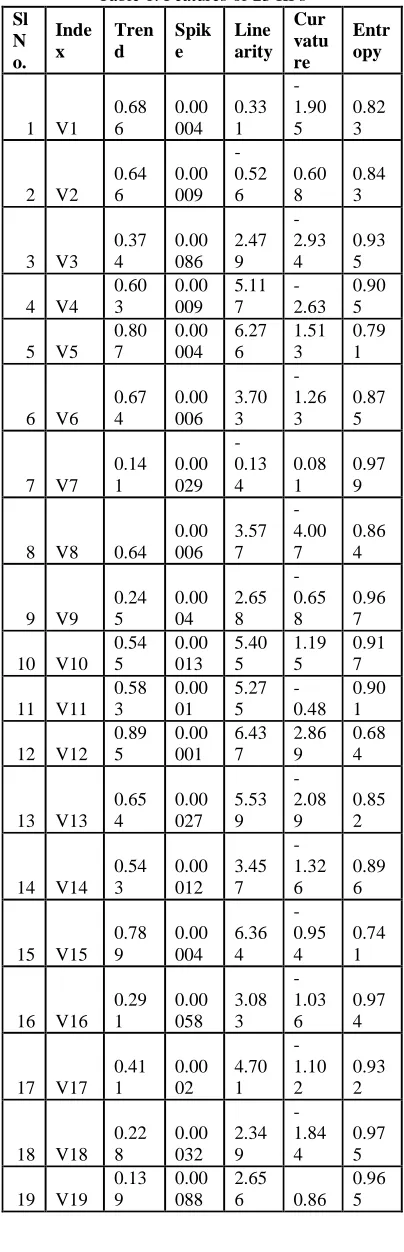
5. DATA ANALYSIS & RESULTS

The extracted features of the twenty three IIPs are given in the following table (Table 1):

Table 1. Features of 23 IIPs

Sl N o. Inde x Tren d Spik e Line arity Cur vatu re Entr opy

1 V1 0.68 6 0.00 004 0.33 1 -1.90 5 0.82 3

2 V2 0.64 6 0.00 009 -0.52 6 0.60 8 0.84 3

3 V3 0.37 4 0.00 086 2.47 9 -2.93 4 0.93 5

4 V4 0.60 3 0.00 009 5.11 7 -2.63 0.90 5

5 V5 0.80 7 0.00 004 6.27 6 1.51 3 0.79 1

6 V6 0.67 4 0.00 006 3.70 3 -1.26 3 0.87 5

7 V7 0.14 1 0.00 029 -0.13 4 0.08 1 0.97 9

8 V8 0.64 0.00 006 3.57 7 -4.00 7 0.86 4

9 V9 0.24 5 0.00 04 2.65 8 -0.65 8 0.96 7

10 V10 0.54 5 0.00 013 5.40 5 1.19 5 0.91 7

11 V11 0.58 3 0.00 01 5.27 5 -0.48 0.90 1

12 V12 0.89 5 0.00 001 6.43 7 2.86 9 0.68 4

13 V13 0.65 4 0.00 027 5.53 9 -2.08 9 0.85 2

14 V14 0.54 3 0.00 012 3.45 7 -1.32 6 0.89 6

15 V15 0.78 9 0.00 004 6.36 4 -0.95 4 0.74 1

16 V16 0.29 1 0.00 058 3.08 3 -1.03 6 0.97 4

17 V17 0.41 1 0.00 02 4.70 1 -1.10 2 0.93 2

18 V18 0.22 8 0.00 032 2.34 9 -1.84 4 0.97 5

19 V19 0.13 9

0.00 088

2.65 6 0.86

0.96 5

20 V20 0.60 7 0.00 016 4.68 3 2.86 9 0.89 2

21 V21 0.55 5 0.00 028 4.93 6 -0.86 1 0.87 9

22 V22 0.83 5 0.00 002 6.22 7 1.42 7 0.75 6

23 V23 0.33 1 0.00 024 2.69 5 2.32 8 0.96 9

The clustering of IIPs on the basis of ‘Trend’ feature is given in the following figure (Fig. 1):

Fig. 1: Clustering of IIPs on Trend The clustering of IIPs on the basis of ‘Spike’ feature is given in the following figure (Fig. 2):

Fig. 2: Clustering of IIPs on Spike The clustering of IIPs on the basis of ‘Linearity’ feature is given in the following figure (Fig. 3):

The clustering of IIPs on the basis of ‘Curvature’ feature is given in the following figure (Fig. 4):

Fig. 4: Clustering of IIPs on Curvature

The clustering of IIPs on the basis of ‘Entropy’ feature is given in the following figure (Fig. 5):

Fig. 5: Clustering of IIPs on Entropy

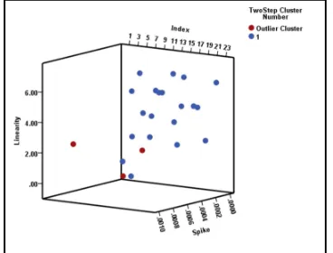
The clustering of the IIPs on the basis of ‘Linearity’ and ‘Spike’ features is shown in the following figure (Fig. 6):

Fig. 6: Clustering of IIPs on Linearity and Spike

6. CONCLUSION

In case of the trend feature, we get two cluster of unequal size, the larger cluster has fourteen (14) indexes and the smaller one has eight (8) while one index was identified as outlier cluster. There are again

two clusters in case of both the spike and linearity features. The larger clusters in both the cases have nineteen (19) indexes and the smaller ones have only three (3). One index is identified as outlier cluster in both the cases. For the curvature feature, we identified two clusters – the larger one with thirteen (13) indexes and the smaller one with nine (9) indexes. In this case also one index is identified as outlier cluster. We have exactly two clusters without any outlier for the entropy feature where the larger one has eighteen (18) indexes and the smaller one has five (5) indexes.

Index V12 is identified as outlier cluster for trend and linearity features, V9 is identified as outlier cluster for spike feature, and V8 is identified as outlier cluster for curvature feature.

We observe that the largest clusters of indexes were exhibited by both the linearity and spike features. Only the entropy feature did not produce any outlier cluster.

The cluster analysis of the indexes together on linearity and spike features produced only one (1) cluster of size twenty (20) with three (3) indexes remained in the outlier cluster. Therefore, we notice that there exist tremendous amounts of hidden pattern in this time series data which may be mined through proper and systematic analyses. This information may be used in the future to develop a useful information system for the interest of the society in large.

REFERENCES

[1] Pan, H., Lin, Z., & Gui, G. (2019). Enabling Damage Identification of Structures Using Time Series–Based Feature Extraction Algorithms.

Journal of Aerospace Engineering, 32(3).

doi:10.1061/(asce)as.1943-5525.0000978 [2] Christ, M., Braun, N., Neuffer, J., &

Kempa-Liehr, A. W. (2018). Time Series FeatuRe Extraction on basis of Scalable Hypothesis tests (tsfresh – A Python package). Neurocomputing,

307, 72-77. doi:10.1016/j.neucom.2018.03.067

[3] Zhang, D., Zuo, W., & Wang, P. (2018). Generalized Feature Extraction for Wrist Pulse Analysis: From 1-D Time Series to 2-D Matrix.

Computational Pulse Signal Analysis, 169-189.

doi:10.1007/978-981-10-4044-3_9

[4] Zang, D., Liu, J., & Wang, H. (2018). Markov chain-based feature extraction for anomaly detection in time series and its industrial application. 2018 Chinese Control And Decision

Conference (CCDC).

doi:10.1109/ccdc.2018.8407286

[5] Karim, F., Majumdar, S., Darabi, H., & Chen, S. (2018). LSTM Fully Convolutional Networks for Time Series Classification. IEEE Access, 6, 1662-1669. doi:10.1109/access.2017.2779939

[6] Katircioglu-Öztürk, D., Güvenir, H. A., Ravens, U., & Baykal, N. (2017). A window-based time series feature extraction method. Computers in

Biology and Medicine, 89, 466-486.

272 [7] Christ, M., Kempa-Liehr, A. W., & Feindt, M.

(2016). Distributed and parallel time series feature extraction for industrial big data applications.

arXiv preprint arXiv:1610.07717.

[8] Ouyang, Z., Sun, X., & Yue, D. (2017). Hierarchical time series feature extraction for power consumption anomaly detection. In

Advanced Computational Methods in Energy, Power, Electric Vehicles, and Their Integration

(pp. 267-275). Springer, Singapore.

[9] Bhardwaj, K., & Marculescu, R. (2017, April). K-hop learning: a network-based feature extraction for improved river flow prediction. In

Proceedings of the 3rd International Workshop on Cyber-Physical Systems for Smart Water Networks (pp. 15-18). ACM.

[10]Wang, H., Li, J., Guo, L., Dou, Z., Lin, Y., & Zhou, R. (2017). Fractal complexity-based feature extraction algorithm of communication signals.

Fractals, 25(04), 1740008.

[11]Cavalcante, R. C., Minku, L. L., & Oliveira, A. L. (2016, July). Fedd: Feature extraction for explicit concept drift detection in time series. In 2016

International Joint Conference on Neural

Networks (IJCNN) (pp. 740-747). IEEE.

[12]Gao, Z. K., Cai, Q., Yang, Y. X., Dang, W. D., & Zhang, S. S. (2016). Multiscale limited penetrable horizontal visibility graph for analyzing nonlinear time series. Scientific reports, 6, 35622.

[13]Susto, G. A., Schirru, A., Pampuri, S., & McLoone, S. (2016). Supervised aggregative feature extraction for big data time series regression. IEEE Transactions on Industrial

Informatics, 12(3), 1243-1252.

[14]Fulcher, B. D., & Jones, N. S. (2016). Automatic time-series phenotyping using massive feature extraction. arXiv preprint arXiv:1612.05296. [15]Das, D., Tripathi, A. K., Shah, A., & Mehta, S.

(2018). Application of Multilayer Perceptron for Forecasting of Selected IIPs of India An Empirical Analysis. International Journal of

Computer Sciences and Engineering, 6(11),

400-406. doi:10.26438/ijcse/v6i11.400406

[16]Cui, Z., Chen, W., & Chen, Y. (2016). Multi-scale convolutional neural networks for time series classification. arXiv preprint arXiv:1603.06995. [17]Liu, R., Meng, G., Yang, B., Sun, C., & Chen, X.

(2017). Dislocated time series convolutional neural architecture: An intelligent fault diagnosis approach for electric machine. IEEE Transactions

on Industrial Informatics, 13(3), 1310-1320.

[18]Yang, J., Nguyen, M. N., San, P. P., Li, X. L., & Krishnaswamy, S. (2015, June). Deep convolutional neural networks on multichannel time series for human activity recognition. In

Twenty-Fourth International Joint Conference on Artificial Intelligence.

[19]Baydogan, M. G., & Runger, G. (2015). Learning a symbolic representation for multivariate time

series classification. Data Mining and Knowledge

Discovery, 29(2), 400-422.

[20]Mörchen, F. (2003). Time series feature extraction for data mining using DWT and DFT. [21]Time series data. (n.d.). Retrieved from:

https://www.ibm.com/support/knowledgecenter/S S3RA7_18.2.0/modeler_mainhelp_client_ddita/co mponents/dt/timeseries_data.html

[22]time series. (n.d.). Retrieved from: http://www.businessdictionary.com/definition/tim e-series.html

[23]Trends. (n.d.) Retrieved from: https://www.ibm.com/support/knowledgecenter/S S3RA7_18.2.0/modeler_mainhelp_client_ddita/co mponents/dt/timeseries_trend.html

[24]Seasonal cycles. (n.d.) Retrieved from: https://www.ibm.com/support/knowledgecenter/S S3RA7_18.2.0/modeler_mainhelp_client_ddita/co mponents/dt/timeseries_seasonal.html

[25]Nonseasonal cycles. (n.d.). Retrieved from: https://www.ibm.com/support/knowledgecenter/S S3RA7_18.2.0/modeler_mainhelp_client_ddita/co mponents/dt/timeseries_nonseasonal.html [26]Pulses and steps. (n.d.). Retrieved from:

https://www.ibm.com/support/knowledgecenter/S S3RA7_18.2.0/modeler_mainhelp_client_ddita/co mponents/dt/timeseries_pulses.html

[27]Outliers. (n.d.). Retrieved from: https://www.ibm.com/support/knowledgecenter/S S3RA7_18.2.0/modeler_mainhelp_client_ddita/co mponents/dt/ts_outliers_overview.html

[28]Trovero, M. A., & Leonard, M. J. (n.d.). Time Series Feature Extraction. Retrieved from https://www.sas.com/content/dam/SAS/support/e n/sas-global-forum-proceedings/2018/2020-2018.pdf.

[29]An Introduction to Clustering and different methods of clustering. (n.d.). Retrieved from: https://www.analyticsvidhya.com/blog/2016/11/a n-introduction-to-clustering-and-different-methods-of-clustering/

[30]Index of industrial production. (2019, January

22). Retrieved from

https://en.wikipedia.org/wiki/Index_of_industrial _production

[31]Trevino, A. (n.d.). Introduction to K-means Clustering. Retrieved from https://www.datascience.com/blog/k-means-clustering

[32]Conduct and Interpret a Cluster Analysis. (n.d.).

Retrieved from

https://www.statisticssolutions.com/cluster-analysis-2/

[33]What is Hierarchical Clustering? (2018, November 07). Retrieved from https://www.displayr.com/what-is-hierarchical-clustering/

273 Platform of India. Released Under: National Data

Sharing and Accessibility Policy (NDSAP). Retrieved from: https://data.gov.in/node/2906361 [35]Monthly indices of all-India Index of Industrial

Production at NIC (2008) 2 digit and Sectoral levels from April 2012 to March 2017. (2017).

Retrieved from

https://data.gov.in/resources/monthly-indices-all- india-index-industrial-production-nic-2008-2-digit-and-sectoral-leve-0

[36]IIP. (n.d.). Retrieved from: https://data.gov.in/keywords/iip