Western University Western University
Scholarship@Western
Scholarship@Western
Electronic Thesis and Dissertation Repository
4-16-2014 12:00 AM
Contextual Anomaly Detection Framework for Big Sensor Data
Contextual Anomaly Detection Framework for Big Sensor Data
Michael Hayes
The University of Western Ontario
Supervisor
Dr. Miriam A.M. Capretz
The University of Western Ontario
Graduate Program in Electrical and Computer Engineering
A thesis submitted in partial fulfillment of the requirements for the degree in Master of Engineering Science
© Michael Hayes 2014
Follow this and additional works at: https://ir.lib.uwo.ca/etd
Part of the Other Electrical and Computer Engineering Commons
Recommended Citation Recommended Citation
Hayes, Michael, "Contextual Anomaly Detection Framework for Big Sensor Data" (2014). Electronic Thesis and Dissertation Repository. 2001.
https://ir.lib.uwo.ca/etd/2001
This Dissertation/Thesis is brought to you for free and open access by Scholarship@Western. It has been accepted for inclusion in Electronic Thesis and Dissertation Repository by an authorized administrator of
(Thesis format: Monograph)
by
Michael A Hayes
Graduate Program in Electrical and Computer Engineering
A thesis submitted in partial fulfillment
of the requirements for the degree of
Masters of Engineering Science
The School of Graduate and Postdoctoral Studies
The University of Western Ontario
London, Ontario, Canada
c
Abstract
Performing predictive modelling, such as anomaly detection, in Big Data is a difficult task.
This problem is compounded as more and more sources of Big Data are generated from
en-vironmental sensors, logging applications, and the Internet of Things. Further, most current
techniques for anomaly detection only consider the content of the data source, i.e. the data
itself, without concern for the context of the data. As data becomes more complex it is
in-creasingly important to bias anomaly detection techniques for the context, whether it is spatial,
temporal, or semantic. The work proposed in this thesis outlines a contextual anomaly
detec-tion framework for use in Big sensor Data systems. The framework uses a well-defined content
anomaly detection algorithm for real-time point anomaly detection. Additionally, we present
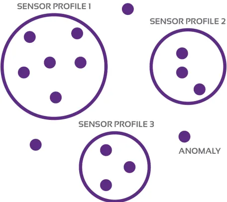
a post-processing context-aware anomaly detection algorithm based onsensor profiles, which are groups of contextually similar sensors generated by a multivariate clustering algorithm. The
contextual anomaly detection framework is evaluated with respect to two different Big sensor
Data datasets; one for electrical sensors, and another for temperature sensors within a building.
The results of the framework were positive in that we were able to detect content anomalies in
real-time, and then pass these anomalies to the context detector. The context detector was able
to reduce the number of false positives identified. Further, the approach is compared against
the R outliers statistical package with positive results.
Keywords: Anomaly detection, point anomalies, context anomalies, Big sensor Data,
pre-dictive modelling, MapReduce
This thesis would not have been made possible without the support and guidance of my friends, family, colleagues, and many others that I have had the pleasure of working with in the past two years. I would first like to thank Dr. Miriam Capretz, Associate Professor in the Department of Electrical and Computer Engineering at Western University and my graduate supervisor for the past two years. I first began working with Dr. Capretz in the final summer of my undergraduate program and she has since been a driving force and motivator in my work. Her guidance, support, and expertise has been hugely important in shaping who I have become. Thank you for your hard work, patience, time, and effort you have given me these past several years.
To my mother, Margaret Fleming, and my father, Robert Hayes, who have given me love, appreciation, and seemingly infinite support throughout my life. You both have had instrumen-tal roles in pushing me to become a better, more well-rounded person. To my brother, David Hayes, I thank you for friendship, motivation, and love. You are a more creative person than I could ever strive to be; I hope I made you proud, brother. Family: I sincerely dedicate this work to you, without all of your help I would not be where I am today.
Vanessa Rusu. You had to deal with a lot these past few years. I thank you for your patience and love, especially through the late nights. You have seen me in my lowest and highest moments, and for that I am deeply grateful. Thank you Vanessa, you were a rock of support for me, and I do not know how I could have possibly done this without you.
I would also like to thank all of the many colleagues I have had the privilege of working with these past two years. David Allison, Kevin Brown, Katarina Grolinger, Wilson Higashino, Abhinav Tiwari, and Alexandra L’Heureux: you all deserve immense credit for helping shape my ideas from random thoughts to directed solutions. I have also had the priviledge of work-ing with many professors, and industry, that have helped shape this thesis and myself as a researcher. To the professors I have had the opportunity to teach with, thank you for having me as a teaching assistant. I hope some of your charm and talent as an educator rubbed offon me. To the members of industry I worked with, thank you for your support and healthy discussions on the application of research in real-world problems.
I would finally like to thank my grandparents, extended family, friends, and others I have missed. I have been fortunate to have some wonderful people in my life, and I thank you for your support.
Contents
Abstract ii
Acknowledgements iii
List of Figures vi
List of Tables vii
List of Listings viii
List of Appendices ix
1 Introduction 1
1.1 Motivation . . . 2
1.2 Thesis Contribution . . . 4
1.3 The Organization of the Thesis . . . 6
2 Background and Literature Review 9 2.1 Concept Introduction . . . 9
2.1.1 Anomaly Detection and Metrics . . . 9
2.1.2 MapReduce . . . 12
2.1.3 Big Data . . . 15
2.2 Anomaly Detection Techniques . . . 17
2.2.1 Bayesian Networks . . . 17
2.2.2 Nearest Neighbour-based Techniques . . . 18
2.2.3 Statistical Modelling . . . 19
2.2.4 Rule-based Techniques . . . 20
2.2.5 Contextual Anomalies . . . 21
2.2.6 Parallel Machine Learning . . . 23
2.3 Anomaly Detection for Big Data . . . 23
2.3.1 Predictive Modelling in Big Data . . . 24
2.3.2 Real-time Analytics in Big Data . . . 27
2.3.3 Computational Complexity . . . 29
2.4 Contextual Anomaly Detection . . . 30
2.4.1 Post-Processing Detection . . . 30
2.4.2 Hierarchical-based Approaches . . . 31
2.5 Summary . . . 33
3.1.1 Hierarchical Approach . . . 34
3.1.2 Contextual Detection Overview . . . 35
3.2 Content Anomaly Detection . . . 37
3.2.1 Univariate Gaussian Predictor . . . 38
3.2.2 Random Positive Detection . . . 39
3.2.3 Complexity Discussion . . . 40
3.3 Context Anomaly Detection . . . 41
3.3.1 Sensor Profiles . . . 41
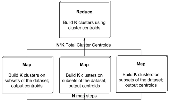
3.3.2 Clustering with MapReduce . . . 42
3.3.3 Multivariate Gaussian Predictor . . . 45
3.3.4 Complexity Discussion . . . 47
3.4 Summary . . . 48
4 Contextual Anomaly Detection Evaluation 50 4.1 Implementation . . . 51
4.1.1 Big Sensor Data . . . 51
4.1.2 Components . . . 54
4.1.3 Virtualized Sensor Stream . . . 59
4.2 Evaluation . . . 60
4.2.1 Dataset 1: Content Detection . . . 60
4.2.2 Dataset 1: Context Detection . . . 62
4.2.3 Dataset 1: Discussion . . . 62
4.2.4 Dataset 2: Content Detection . . . 63
4.2.5 Dataset 2: Context Detection . . . 64
4.2.6 Dataset 2: Discussion . . . 66
4.2.7 Random Positive Detection . . . 67
4.2.8 Comparison With Other Algorithms . . . 68
4.3 Summary . . . 68
5 Conclusion and Future Work 70 5.1 Conclusion . . . 70
5.2 Future Work . . . 72
Bibliography 76
A Big Sensor Data Examples 80
Curriculum Vitae 81
List of Figures
2.1 Types of Anomalies . . . 11
2.2 Sensitivity and specificity matrix defining the relationships between a test out-come and the expected condition. . . 13
2.3 Classic 3 V’s of Big Data: Velocity, Volume, and Variety. . . 16
2.4 Bayesian Network Examples. The subcaptions indicate the formula to calculate the overall probability for each network. . . 18
2.5 Decision-tree Rule-based Classification . . . 21
3.1 Contextual Anomaly Detection Framework Hierarchy . . . 35
3.2 Contextual Anomaly Detection Framework . . . 36
3.3 Sensor Profile Definition . . . 43
3.4 MapReduce to Determine Global Sensor Labels . . . 44
3.5 MapReduce to Re-label Sensors to Global Sensor Profiles . . . 45
4.1 Big Sensor Data Case Study . . . 52
4.2 Frequency Histogram for Evaluation Data . . . 55
4.3 Content Detection for Dataset 1: the black diamonds represent a sensor read-ing instance, and the grey lines connect continuous readread-ing instances. The highlighted portion at the top represents those reading instances identified as anomalous with respect to content. . . 61
4.4 Content Detection for Dataset 2: the black diamonds represent reading stances. The top and bottom highlighted portions in grey identify reading in-stances that were considered anomalous with respect to their content. . . 65
4.5 Context Detection for Datasets 1 and 2 . . . 67
4.6 Average Density of Data Found by R . . . 69
4.7 R Results: Graphical Representation . . . 69
2.1 Anomaly Detection Definitions . . . 10
2.2 Anomaly Detection Types Definitions . . . 12
2.3 Sensitivity and Specificity Definitions . . . 13
2.4 Definitions for Types of Contextual Attributes . . . 22
3.1 Context Examples . . . 42
4.1 Sensor Dataset and Corresponding Domains . . . 53
4.2 Sensor Associated Meta-Information . . . 54
4.3 Sensor Dataset 1: HVAC . . . 60
4.4 Dataset Example . . . 61
4.5 Dataset 1 Running Time Results . . . 62
4.6 Anomalous Examples for Dataset 1 . . . 63
4.7 Sensor Dataset 2: Temperature . . . 64
4.8 Dataset Example . . . 64
4.9 Dataset 2 Running Time Results . . . 66
4.10 Anomalous Examples for Dataset 2 . . . 66
4.11 Results Comparison between the CADF and R Outliers Package . . . 69
List of Listings
2.1 Code Snippet for a Simple Map and Reduce Operation . . . 14
4.1 Code Snippet to Build the Real-Time Model . . . 55
4.2 Code Snippet to Evaluate the Real-Time Model . . . 56
4.3 Code Snippet to Build the Multivariate Gaussian Model . . . 57
4.4 Code Snippet to Evaluate the Multivariate Gaussian Model . . . 58
4.5 Code Snippet for Virtualized Sensor Stream . . . 59
4.6 Code Snippet for Including Randomized Positive Detection . . . 67
Appendix A Big Sensor Data Examples . . . 80
Chapter 1
Introduction
Anomaly detection is the identification of abnormal events or patterns that do not conform to
expected events or patterns[15]. Detecting anomalies is important in a wide range of disparate
fields, such as, diagnosing medical problems, bank and insurance fraud, network intrusion,
and object defects. Generally anomaly detection algorithms are designed based on one of
three categories of learning: unsupervised, supervised, and semi-supervised[15]. These
tech-niques range from training the detection algorithm using completely unlabelled data to having
a pre-formed dataset with entries labelled normal or abnormal. A common output of these techniques is a trained categorical classifier which receives a new data entry as the input, and
outputs a hypothesis for the data points abnormality.
Anomaly detection can be divided into detection of three main typesof anomalies: point, collective, and contextual. Point anomalies occur when records are anomalous with respect to
all other records in the dataset. This is the most common type of anomaly and is well-explored
in literature. Collective anomalies occur when a record is anomalous when considered with
adjacent records. This is prevalent in time-series data where a set of consecutive records are
anomalous compared to the rest of the dataset. The final type, contextual, occurs when a
record is only considered anomalous when it is compared within the context of other
meta-information. Most research focuses on the former two types of anomalies with less concern
for the meta-information. However, in domains such as streaming sensor applications,
anoma-lies may occur with spatial, temporal, dimensional, or profile localities. Concretely, these are
localities based on the location of the sensor, the time of the reading, the meta-information
associated with the sensor, and the meta-information associated with groups of sensors. For
example, a sensor reading may determine that a particular electrical box is consuming an
ab-normally high amount of energy. However, when viewed in context with the location of the
sensor, current weather conditions, and time of year, it is well within normal bounds.
1.1
Motivation
One interesting, and growing, field where anomaly detection is prevalent is inBig sensor Data. Sensor data that is streamed from sources such as electrical outlets, water pipes,
telecommu-nications, Web logs, and many other areas, generally follows the template of large amounts of
data that is input very frequently. In all these areas it is important to determine whether faults
or defects occur. In electrical and water sensors, this is important to determine faulty sensors,
or deliver alerts that an abnormal amount of water is being consumed, as an example. In Web
logs, anomaly detection can be used to identify abnormal behavior, such as identify fraud. In
any of these cases, one difficulty is coping with the velocity and volume of the data while still
providing real-time support for detection of anomalies. Further, organizations that supply
sen-soring services compete in an industry that has seen huge growth in recent years. One area that
these organizations can exploit to gain market share is through providing more insightful
ser-vices beyond standard sensoring. These insightful serser-vices can include energy trends, anomaly
detection, future prediction, and usage reduction approaches. All of this culminates in a future
that includes smart buildings: that is, buildings that can manage, optimize, and reduce their
own energy consumption, based on Big sensor Data [14].
The amount of data produced by buildings, organizations, and people in general, is
1.1. Motivation 3
intelligent decision making systems. This is because many decision making algorithms exploit
the idea that more data to train the algorithm creates a more accurate model. A caveat is that
this does not hold for algorithms that suffer from high bias [20]. However, algorithms that are
highly biased can be improved upon through adding extra features; this is common in highly
widedatasets, where there exists a large number of features. With all the benefits of Big Data and predictive modelling, there are certainly some drawbacks. One of the major constraints is
in feature selection. As in most machine learning approaches, selecting the features which best
represent the data model is a difficult task.
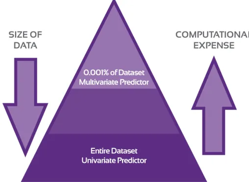
Along similar lines, another major constraint is in the types of algorithms used for
predic-tive modelling in general, and thus anomaly detection as a subset of predicpredic-tive modelling. Some
consider that there is a paradigm shift in the types of algorithms used: from computationally
expensive algorithms to computationally inexpensive algorithms. The inexpensive algorithms
may have much higher training accuracy error; that is, the error accumulated per record when
training. However, when normalized over the entire, large, dataset, the higher training accuracy
error converges to a lesser prediction error. Prediction error is defined as the error accumulated
when predicting new values from a trained predictor [18]. The prediction error for the
inexpen-sive algorithm is within similar ranges as those found with the computationally more expeninexpen-sive
algorithm, yet occurring over a much smaller time frame. A motivation of this work is to then
take this idea and shift it to incorporate these computationally expensive algorithms which still
generally perform better. By applying a hierarchical approach which involves only calculating
the expensive algorithm on a very small subset of the initial data, the approach can utilize the
best of both worlds.
Real-time detection for Big Data systems is also a growing area of interest. One of the
common attributes associated with Big Data isvelocity. Velocity is not only the rate at which data is input to the system, but also the rate at which the data can be processed by the system.
Ensuring algorithms can process data in real-time is not an easy task as many require huge
such as data visualization where real-time feedback by the user is important in skewing the
algorithm to presenting appropriate visualizations. Data visualization is also a common method
for determing anomalous values. Therefore, a motivation of this work is to present a framework
that can cope with Big Data in real-time; while not neccessarily for data visualization, but for
identification of real-time anomalies as they are streamed to the framework.
An area that has not been well explored in literature is contextual anomaly detection for
sensor data. Some related works have focused on anomaly detection in data with spatial
relationships[27], while others propose methods to define outliers based on relational class
attributes [36]. A prevalent issue in these works is their scalability to large amounts of data. In
most cases the algorithms have increased their complexity to overcome more naive methods,
but in doing so have limited their application scope to offline detection. This problem is
com-pounded as Big Data requirements are found not only in giant corporations such as Amazon or Google, but in more and more small companies that require storage, retrieval, and querying
over very large scale systems. As Big Data requirements shift to the general public, it is
im-portant to ensure that the algorithms which worked well on small systems can scale out over
distributed architectures, such as those found in cloud hosting providers. Where an algorithm
may have excelled in its serial elision, it is now necessary to view the algorithm in
paral-lel; using concepts such as divide and conquer, or MapReduce[19]. Many common anomaly
detection algorithms such as k-nearest neighbour, single class support vector machines, and
outlier-based cluster analysis are designed for single machines [45]. A main goal of this
re-search is to leverage existing, well-defined, serial anomaly detection algorithms and redefine
them for use in Big Data analytics.
1.2
Thesis Contribution
There are a number of contributions for the work presented in this thesis; this section
1.2. ThesisContribution 5
extendible, and scalable framework for contextual anomaly detection in Big sensor Data. We
confine the contribution of this work to Big sensor Data; however, the framework is generalized
such that any application which hascontextualattributes andbehaviouralattributes can utilize the framework. An additional contribution is the ability to apply the framework to real-time
detection of algorithms for use in Big sensor Data applications. We also stress that the
frame-work presented is modular in its architecture, allowing the content and contextual detection
algorithms be replaced by new research.
The second contribution is to provide a paradigm shift in the way algorithms are structured
for Big Data. As research has progressed in the machine learning domain, and in particular
the anomaly detection domain, algorithms become more and more computationally expensive,
and accurate. Thus, another contribution of this work is to provide a hierarchical approach to
algorithm construction for Big Data; where a computationally inexpensive, inaccurate, model
is used to first determine initial anomalies. From this smaller pool of records, the
computation-ally more expensive model can be used to reduce the number of false positives generated by
the first model. This hierarchical model can be used in many other domains; here we present a
framework for exposing this model specifically for Big sensor Data. The modularity presented
in the first contribution also is tied into this hierarchical structure. Due to the separation of
concerns existing within the framework, the modules can be independently created, merged,
modified, and evaluated without effecting the other modules. This also means additional
mod-ules can be added to the framework, such as semantic detection algorithms, to further enhance
the framework.
In summary, the thesis will describe a technique to detect contextually anomalous values in
streaming sensor systems. This research is based on the notion that anomalies have dimensional
and contextual locality. That is, the dimensional locality will identify those abnormalities
which are found to be structurally different based on the sensor reading. Contextually, however,
the sensors may introduce new information which diminishes or enhances the abnormality of
night for electrical sensor data; however, when introduced with context such as time of day,
and building business hours, anomalous readings may be found to be false positives.
To cope with the volume and velocity of Big Data, the technique will leverage a parallel
computing model, MapReduce. Further, the technique will use a two-part detection scheme
to ensure that point anomalies are detected in real-time and then evaluated using contextual
clustering. The latter evaluation will be performed based onsensor profileswhich are defined by identifying sensors that are used in similar contexts. The primary contribution of this
tech-nique is to provide a scalable way to detect, classify, and interpret anomalies in sensor-based
systems. This ensures that real-time anomaly detection can occur. The proposed approach is
novel in its application to very large scale systems, and in particular, its use of contextual
in-formation to reduce the rate of false positives. Further, we posit that our work can be extended
by defining a third step based on the semantic locality of the data, providing a further reduction
in the number of anomalies which are false positive.
The results of the implementation for this research are positive. The framework is able
to identify content anomalies in real-time for a real-world dataset and conditions. Further,
the number of false positives identified by the content detector are reduced when passed to
the context detector. Also, the framework has been compared against the R statistical outliers
package with positive results: the anomalies identified by the framework are equivalent to those
identified by R.
1.3
The Organization of the Thesis
The remainder of this thesis is organized as follows:
• Chapter 2 outlines both the background information associated with contextual anomaly
detection for Big sensor Data, and a ltierature review of the current approaches to
contex-tual anomaly detection for Big sensor Data. This chapter will first provide an introduction
1.3. TheOrganization of theThesis 7
overview of practical approaches for anomaly detection will be explored, including an
introduction to a variety of algorithms with their benefits and drawbacks. Finally, the
chapter will provide a review of state of the art techniques presented in academia for
contextual anomaly detection, and anomaly detection in Big Data.
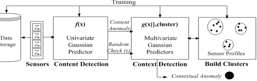
• Chapter 3 contains the main contribution for this thesis. The chapter will provide a
de-scription of the components for the Contextual Anomaly Detection Framework (CADF).
Included in the description is an overview of each individual components, and how
they interact with one another. The chapter is broken into two components: the
con-tent anomaly detector and the context anomaly detector. The concon-tent anomaly detection
section includes information on the algorithm used by the detector, the random positive
detection component, and a complexity discussion to provide insight into the scalability
for Big Data. The context anomaly detection section provides detail on generating the
Sensor Profiles (SPs) using the MapReduce framework, the underlying context detection
algorithm, and a complexity discussion. Finally, a summary of how the components
in-teract with each other, and how their inin-teraction provides modularity and scalability for
Big Data is presented.
• Chapter 4 includes a description of the implementation and evaluation of the CADF.
First, the implementation for each component of the CADF will be shown. In particular,
a look at the types of datasets that can be evaluated by the implementation is presented.
Finally, how the components will interact with each other in a virtualized sensor stream
will be explored. This final discussion is important as the case studies that will be
dis-cussed in the evaluation section are offline datasets that are exported from real-world data
streams. To be consistent with the real-world counterpart, the virtualized sensor stream
was created. The second major section of this chapter is focused on the evaluation of the
CADF implementation. This portion of the chapter involves describing the streaming
with some offline anomaly detection algorithms is shown.
• Chapter 5 provides the conclusion for this work, as well as a discussion on possible
Chapter 2
Background and Literature Review
The goal of this chapter is two-fold: first, the concepts that will be explored in the proposed
work will be discussed; second, an overview of the related research works for contextual
anomaly detection will be presented. The literature review will include works specifically
related to contextual detection inBig Data, but also for contextual detection for standard sized data.
2.1
Concept Introduction
This section will introduce concepts and terminology related toanomaly detection,
MapRe-duce, Big Data,andcontext. These concepts will first be defined, and then discussed in the
context of academia and implementation practice. Therefore, this section serves as a primer
for the concepts that will be explored further in the rest of the thesis.
2.1.1
Anomaly Detection and Metrics
Anomaly detection can be categorized by three attributes:input data, availability of data labels (anomalous versus normal), anddomain specific restraints[34]. To begin, Table 2.1 introduces common terminology that is used to describe the first attribute: input data. One of the major
considerations in using an anomaly detection algorithm is based on the type of features present
within the set of records, i.e. categorical, continuous, and binary. Further, another
considera-tion are the relaconsidera-tionships existing within the data itself. Many applicaconsidera-tions assume that there
exist no relationships between the records; these are generally consideredpointanomaly sce-narios. Other applications assume that relationships may exist; these are generally referreed
to as contextual anomalies. The types of anomalies that may occur are discussed further in Table 2.2 [15].
Term Definition
Record A data instance; for example: sensor data including the reading,
location, and other information.
Feature The set of attributes to define the record; for example: the reading, and location are each individual features.
Binary Feature The feature can be of a binary number of possible values.
Categorical Feature The feature can be of a categorical number of possible values; for example: a direction feature may be categorical with the set of values north, south, east and west.
Continuous Feature The feature can be of a continuous number of possible values; for example: the sensor reading may be any floating point number [0, 100].
Univariate The record is composed of a single feature.
Multivariate The record is composed of several features.
Table 2.1: Anomaly Detection Definitions
Algoritms aimed at detecting anomalies can be categorized based on the types of data labels
known apriori. Namely, if the algorithm knows a set of records is anomalous, it is referred to
as asupervisedlearning algorithm. In contrary, if the algorithm has no notion of the labels of data, anomalous or otherwise, the algorithm is referred to as aunsupervisedlearning algorithm. Further, a third category titledsemi-supervised learning algorithms, involves approaches that assume the training data only has labelled instances for thenormal datatype. This is a more
common approach to anomaly detection thansupervisedlearning algorithms as it is norrmally difficult to wholly identify all the abnormal classes [25]. However, the most common approach
2.1. ConceptIntroduction 11
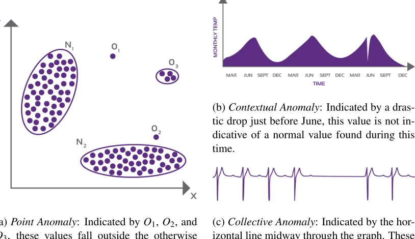
(a)Point Anomaly: Indicated by O1,O2, and
O3, these values fall outside the otherwise
dense regions ofN1andN2.
(b)Contextual Anomaly: Indicated by a dras-tic drop just before June, this value is not in-dicative of a normal value found during this time.
(c)Collective Anomaly: Indicated by the hor-izontal line midway through the graph. These values are all anomalous when considered contiguously against the normal pattern of the rest of the data.
Figure 2.1: Types of Anomalies
types of algorithms relies on the assumption that anomalies are far less frequent than normal
records in the dataset. Further, an underlying assumption in most of these algorithms,
regard-less of category, is that they rely on the assumption that anomalies are dynamic in behavior.
That is, it is very difficult to determine all thelabelsof anomalies for the entire dataset, and the future direction the dataset will take. Finally, most anomaly detection applications in practice
have the anomalous and normal labels defined through human effort. As a result, it is much
more common in practice to find datasets which are wholly unlabelled, or partially unlabelled,
requiring the use of an unsupervised or semi-supervised learning algorithm [44].
This chapter will also introduce concepts related to some metrics used in the contribution
and evaluation chapters: Chapter 3, and Chapter 4 respectively. The first concepts to introduce
are related tosensitivityandspecificity[31]. These are metrics used within classification tests to determine how well a classifier performs in classifying the correct versus incorrect errors.
Term Definition
Point Anomalies A single record is considered to be abnormal with respect to the other records in the dataset. Point anomalies are the most com-mon application for anomaly detection, and research in anomaly detection, as will be shown in Section 2.2. A web server identifies a user as a victim of identity theft based on anomalous web page visits. A pictorial example is shown in Figure 2.1a.
Contextual Anomalies A record is anomalous within a specific context. For example, a sensor reading may only be considered anomalous when evalu-ated in the context of temporal and spatial information. A reading value of zero may be anomalous during normal working hours for a business, but non-anomalous during off-work hours. Pictorally this is shown in Figure 2.1b.
Collective Anomalies A single record is considered collectively anomalous when con-sidered with respect to the entire dataset, an example is shown in Figure 2.1c. Concretely, this means that the record may not be considered as anomalous alone; however, when combined within a collective of sequential records, it may be anomalous.
Table 2.2: Anomaly Detection Types Definitions
the definitions for specificity and sensitivity, they will make use of the terms that are used to
define these terms; namely,false positives, false negatives, true positives,andtrue negatives.
The term chart, Table 2.3, can also be explained more clearly through a figure, as shown in
Figure 2.2.
2.1.2
MapReduce
MapReduce is a programming paradigm for processing large datasets in distributed
environ-ments [17] [19]. In the MapReduce paradigm, theMapfunction performs filtering and sorting operations, while the Reduce function carries out grouping and aggregation operations. The classicHello, World! example for MapReduce is shown in Listing 2.1. In the example, the
Map function splits the document into words, and produces a key-value pair for each word in the document. The Reducefunction is responsible for aggregating the output of the Map
2.1. ConceptIntroduction 13
Term Definition
Sensitivity orrecall rate The proportion of actual positives identified as positive. Specificity ortrue negative rate The proportion of actual negatives identified as negative.
True Positive (TP) Positive examples identified as positive.
True Negative (TN) Negative examples identified as negative.
False Positive (FP) Negative examples identified as positive.
False Negative (FN) Positive examples identified as negative.
Table 2.3: Sensitivity and Specificity Definitions
Figure 2.2: Sensitivity and specificity matrix defining the relationships between a test outcome and the expected condition.
in this example partialCounts. The Reduce function groups by word and sums the values received in thepartialCountslist to calculate the occurrence for each word.
The main contribution of MapReduce paradigm is the scalability as it allows for highly
par-allelized and distributed execution over large number of nodes. In the MapReduce paradigm,
the map or the reduce task is divided into a high number of jobs which are assigned to nodes
in the network. Reliability is achieved by reassigning failed nodes job to another node. A well
known open source MapReduce implementation is Hadoop which implements the MapReduce
programming paradigm on top of the Hadoop Distributed File System (HDFS) [11], which is
machine learning algorithms, anomaly detection as an example, is to aid in scaling the machine
learning algorithms toBig Data. .
Listing 2.1: Code Snippet for a Simple Map and Reduce Operation
function map(name, doc) {
for(word : doc)
emit(word, 1);
}
function reduce(word, List partialCounts) {
sum = 0;
for(pc : partialCounts)
sum += pc;
emit(word, sum);
}
While there exists an appeal for MapReduce in scaling machine learning algorithms for
Big Data, there also exist many issues. Specifically, when considering the volume component of Big Data, additional statistical and computational challenges are revealed [22]. Regardless
of the paradigm used to develop the algorithms, an important determinant of the success of
supervised machine learning techniques is the pre-processing of the data [35]. This step is
often critical in order to obtain reliable and meaningful results. Data cleaning, normalization,
feature extraction and selection are all essential in order to obtain an appropriate training set.
This poses a massive challenge in the light of Big Data as the preprocessing of massive amounts
of tuples is often not possible.
More specifically, in the domain of anomaly detection and predictive modelling,
MapRe-duce has a major constraint which limits its usefulness when predicting highly correlated data.
MapReduce works well in contexts where observations can be processed individually [38]. In
2.1. ConceptIntroduction 15
correlated observations that need to be processed together, MapReduce offers little benefit over
non-distributed architectures. This is because it will be quite common that the observations
that are correlated are found within disparate clusters, leading to large performance overheads
for data communication. Use cases such as this are commonly found in predicting stock market
fluctuations. To allow MapReduce to be used in these types of predictive modeling problems,
there are a few potential solutions based on solutions from predictive modeling on traditional
data sizes: data reduction, data aggregation, and sampling. Therefore, it is important to select
aspects of the machine learning algorithm or framework to implement MapReduce efficiently
and effectively.
2.1.3
Big Data
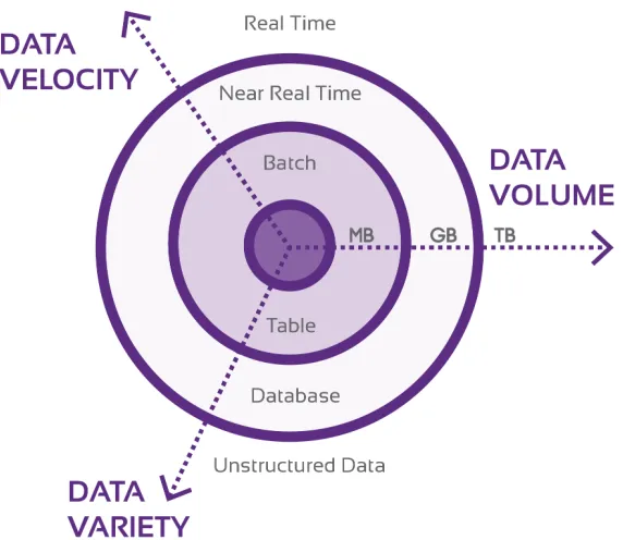
Big Datacan be defined as massive and complex datasets composed of a variety of data struc-tures, including structured, semi-structured, and unstructured data. Big Data was originally
defined by the Gartner group as the three V’s: volume, velocity, and variety [46]. In recent
years, additional ”V’s” have been added to include: veracity, value, and visualization to cope
with the evolving requirements of organizational benefits for addressing and understanding
Big Data. Currently, businesses are acutely aware that huge volumes of data, which continue
to grow, can be used to generate new valuable business opportunities through Big Data
pro-cessing and analysis [43]. Figure 2.3 illustrates the evolution of the three standard V’s of Big
Data.
Velocity refers to processing Big Data with speeds of real-time or near real-time. Velocity
is also related to the rate of changes within the data; that is, data may be processed in bursts
of entries, rather than at constant rates. This is important in many anomaly detection domains
where the anomalies cause a reactionary effect. For example, in systems with complex event
processing, the anomaly detection component can fire events for the complex event processor
to react to. The reaction may be optimizing a cloud network that the complex event processor
Figure 2.3: Classic 3 V’s of Big Data: Velocity, Volume, and Variety.
energy [23].
Volume refers to the growing amount of data stored, from megabytes to pentabytes and
be-yond. The volume of data is important in the sensoring domain as normal operating parameters
for sensor applications are thousands of sensors per location, each streaming sensor readings
every minute. Within a company’s storage system there may also exist hundreds or thousands
of clients with several locations. This culminates in a huge volume of data being stored.
Variety refers to the component of Big Data that includes the requirement to store disparate
datatypes such as: tables, other databases, photos, web data, audio, video, unstructured data,
social media, and primitive datatypes such as integers, floats, and characters. Within the
sen-soring domain this is also important as sensors exist for a variety of sources, such as lighting,
heating and ventillation, greenhouse gas emissions, hydro, and waste control. Further,
sensor-ing companies also store audio, images, video, and demographic information related to their
clients. Additionally, sensor networks may evolve overtime, resulting in a fluid data schema
2.2. AnomalyDetectionTechniques 17
2.2
Anomaly Detection Techniques
In this section, various anomaly detection techniques will be presented that are generally used
for detecting anomalies in streaming sensor networks. In particular, this section will describe
the prosand consof each approach in general. Further, this section will serve as a basis for why the algorithm for the contribution is selected in Chapter 3. There are some challenges
for anomaly detection in sensor networks, namely, the prescence of noise in the data makes
anomaly detection more challenging, and data is collected from distributed, disparate, sources.
As a result, the approaches that will be discussed are:
• Bayesian Networks.
• Parametric Statistical Modelling.
• Nearest Neighbour-based Techniques.
• Rule-based Techniques.
2.2.1
Bayesian Networks
Bayesian networks are commonly used in multi-class anomaly detection scenarios. Bayesian
networks are a classification-based approach whereby the network estimates the probability of
observing a class label given a test record. The class label with the highest probability is
cho-sen as the predicted class label for the test record. An example of a Bayesian network is shown
in Figure 2.4. There are a few advantages to the classification-based Bayesian network
ap-proach. First, multi-class Bayesian networks use a powerful algorithm to distinguish between
instances belonging to different classes. Second, the testing phase is fast. This is important in
anomaly detection for sensor networks as real-time evaluation forallthe sensor readings must be processed. Without a real-time testing phase, this is impossible.
Bayesian networks also have some disadvantages for anomaly detection that eliminate them
Figure 2.4: Bayesian Network Examples. The subcaptions indicate the formula to calculate the overall probability for each network.
multiple anomaly class labels or multiple normal class labels, rely on the readily available class
labels for all the normal classes. As was previously discussed, this is generally not possible for
practical purposes. Human intervention is normally required to label training records, which
is not always available. Second, Bayesian approaches assign discrete labels to the test record.
This is not disadvantageous for sensor networks as meaningful anomaly score is not always required. However, when evaluating the effectiveness of the anomaly detection approach, it is
useful to discriminate between anomaly scores. This is more evident inBig Datacontexts as a continuous anomaly score can aid in reducing the overall number of anomalies needing to be
evaluted.
2.2.2
Nearest Neighbour-based Techniques
Nearest neighbour-based techniques rely on a single underlying assumption: normal data
records occur in dense neighbourhoods, while anomalies occur far from their closest
neigh-bours. The major consideration for nearest neighbour-based approaches is that a distance, or
similarity, metric must be defined for comparing two data records. For some datasets this is
simple; for example, continuous features can be evaluated with Euclidean distance. For
cate-gorical attributes, pairwise comparison of the feature can be used. For multiple features, each
feature is compared individually and then aggregated. One of the main advantages of such an
considera-2.2. AnomalyDetectionTechniques 19
tion for anomaly detection in Big sensor Data is that it is difficult to label the training data.
For nearest neighbour-based techniques this is not necessary. Using nearest neighbour-based
techniques is normally straightforward and only requires the definition of a similarity metric.
The definition of the similarity metric is one of the major drawbacks for nearest
neighbour-based approaches. In many cases, including the Big sensor Data scenario, it is very difficult
to determine a suitable similarity metric for the aggregation and variety of unstructured,
semi-structured, and structured data. The performance of nearest neighbour-based approaches relies
heavily on the similarity metric, and thus when it is difficult to determine the distance measure,
the technique performs poorly. Further, as in all unsupervised techniques, if there is not enough
similar normal data, then the nearest neighbour-based technique will miss anomalies. The biggest problem with nearest neighbour-based approaches is the computational complexity in
evaluating the similarity metric for test records. Namely, the simliarity metric needs to be
computed for the test record to all instances belonging to the training data to compute the
nearest neighbours. This also needs to be done foreverytest data, an extremely difficult task for real-time evaluation of thousands of streaming sensor readings.
2.2.3
Statistical Modelling
Statistical modelling approaches rely on the assumption that normal records occur in high
probability regions of a stochastic model, while anomalies occur in the low probability region.
These techniques fit a statistical model to the given training dataset and then apply a
statisti-cal inference model to determine if the test record belongs to the model with high probability.
There are two types of statistical modelling techniques: parametric and non-parametric models.
Parametric techniques assume that normal data is generated by a parametric distribution, such
an example is the Gaussian model and the Regression model. Non-parametric techniques make
few assumptions about the underlying distribution of the data and include techniques such as
histogram-based, and kernel-based approaches. There are several advantages to the
First, if assumptions hold true then the approach provides a statistically justified solution to the
problem. Second, the anomaly score output by the statistical model can be associated with a
confidence interval which can be manipulated by the algorithm. This provides additional
in-formation for the algorithm to use to improve the efficiency and performance of the algorithm.
Finally, the Big sensor Data context normally follows a normal, or Gaussian, distribution.
However, there are several disadvantages to the statistical modelling approach. First, if the
underlying assumption of the data being distributed from a particular distribution fails then the
statistical technique will fail. Second, selecting the test hypothesis is not a straightforward task
as there exists several types of test statistics. While these disadvantages certainly effect the
Big sensor Data scenario, there are ways to overcome the disadvantages while retaining the
aforementioned advantages. For example, evaluating the algorithm with respect to a variety of
test statistics can be done apriori. Comparing the results of this step will allow the algorithm
to selec the most appropriate test statistic for the given use case.
2.2.4
Rule-based Techniques
Rule-based techniques are quite similar in their disadvantages and advantages to the Bayesian
network technique. Rule-based techniques focus on learning rules that capture the normal
im-plementation of the system. When testing a new value, if there does not exist a rule to
encom-pass the new value, it is considered anomalous. Rules can have associated confidence intervals
which normalizes the proportion between the number of training cases evaluated correctly by
the rule to the total number of training cases covered by the rule. The most obvious benefit
of taking a rule-based approach is that the rules represent real-world reasonings behind why a
value is anomalous. This is in stark constrast to some of the other approaches, such as
statis-tical modelling, which provide parameters that mean little to a human observer. Further, like
Bayesian networks, a rule-based approach shines since it only needs to compare itself with the
existing rules, resulting in a fast testing time. This is especially true for rule-based approaches
2.2. AnomalyDetectionTechniques 21
example of a decision-tree approach is shown in Figure 2.5.
However, like Bayesian networks, there exist some major disadvantages to the rule-based
approach. First, rule-based approaches rely heavily on apriori knowledge of training records
that are anomalous versus normal. In slight contrast to Bayesian networks, rule-based networks
especially need a detailed set of training records which are considered as normal to ensure a
sufficient set of rules are determined. Second, while it was previously mentioned that
rule-based approaches are fast to test, this may not always be the case when there exists a large,
complex, set of rules. Determining the number and complexity of the rules in a rule-based
sys-tem is an important consideration. Too complex and the syssys-tem performs with less efficiency;
not enough complexity and the system provides a large number of false positives and false
negatives.
Figure 2.5: Decision-tree Rule-based Classification
2.2.5
Contextual Anomalies
Contextual anomalies are considered in applications where the dataset has a combination of
contextual attributes and behaviour attributes. These terms are sometimes referred to as
envi-ronmental and indicator attributes, as introduced by Song et al [48]. There are generally four
common ways in which we define contextual attributes, these are defined in Table 2.4.
Contextual anomaly applications are normally handled in one of two ways. First, the
Term Definition
Spatial The records in the dataset include features which identify loca-tional information for the record. For example, a sensor reading may have spatial attributes for the city, province, and country the sensor is located in; it could also include finer-grained informa-tion about the sensors locainforma-tion within a building, such as floor, room, and building number.
Graphs The records are related to other records as per some graph struc-ture. The graph structure then defines a spatial neighbourhood whereby these relationships can be considered as contextual indi-cators.
Sequential The records can be considered as a sequence within one another. That is, there is meaning in defining a set of records that are posi-tioned one after another. For example, this is extremely prevalent in time-series data whereby the records are timestamped and can thus be positioned relative to each other based on time readings. Profile The records can be clustered within profiles that may not have
explicit temporal or spatial contextualities. This is common in anomaly detection systems where a company defines profiles for their users; should a new record violate the existing user profile, that record is declared anomalous.
Table 2.4: Definitions for Types of Contextual Attributes
attempts to apply separate point anomaly detection techniques to the same dataset, within
dif-ferent contexts. This requires a pre-processing step to determine what the contexts actually are,
what the groupings of anomalies within the contexts are, and classifying new records as falling
within one of these contexts. In the first approach, it is necessary to define the contexts of
normal and anomalous records apriori, which is not always possible within many applications.
This is true for the Big sensor Data use case, where it is difficult to define the entire set of
known anomalous records.
The second approach to handling contextual anomaly applications is to utilize the existing
structure within the records to detect anomalies using all the data concurrently. This is
espe-cially useful when the context of the data cannot be broken into discrete categories, or when
new records cannot easily be placed within one of the given contexts. The second approach
2.3. AnomalyDetection forBigData 23
algebra in calculating a contextual anomaly is computationally expensive. The most common
approach to handling contextual anomalies is to reduce the problem into a point anomaly
prob-lem.
2.2.6
Parallel Machine Learning
When discussing anomaly detection algorithms in the context of Big Data it is important to
note programming paradigms that have been developed to handle Big Data efficiently. Srinivas
et al. [2] and Srirama et al. [49] both illustrate the importance and use of MapReduce as a
pro-gramming paradigm for efficient, parallel, processing of Big Data. Efficient processing of Big
Data is important because real-time predictive models are already well-established for smaller
datasets. Therefore, future predictive models should conserve the ability to build real-time
pre-dictors when moving to larger volumes of data. Programming paradigms to achieve this have
been seen in some popular software products such as Mahout [5], HaLoop [12], Spark [6], and
Pregel [40]. These products attempt to scale machine learning algorithms (including predictive
modeling techniques) to multi-machine architectures. However, there is still a research gap
in addressing novel algorithms that are optimized specifically for predictive modeling in Big
Data.
2.3
Anomaly Detection for Big Data
Anomaly detection algorithms in academia can be broadly categorized as point anomaly
de-tection algorithms and context-aware anomaly dede-tection algorithms[15]. Contextual anomalies
are found in datasets which include both contextual attributes and behavioral attributes. For
example, environmental sensors generally include the sensor reading itself, as well as spatial
and temporal information for the sensor reading. Many previous anomaly detection algorithms
in the sensoring domain focus on using the sequential information of the reading to predict
propose a data-driven modelling approach to identify point anomalies in such a way. In their
work they propose severalone-step ahead predictors; i.e. based on a sliding window of pre-vious data, predict the new output and compare it to the actual output. Hill and Minsker [29]
note that their work does not easily integrate several sensor streams to help detect anomalies.
This is in contrast to the work outlined in this thesis where the proposed technique includes a
contextual detection step that includes historical information for several streams of data, and
their context.
In an earlier work, Hill et al. [30] proposed an approach to use several streams of data
by employing a real-time Bayesian anomaly detector. The Bayesian detector algorithm can
be used for single sensor streams, or multiple sensor streams. However, their approach relies
strictly on the sequential sensor data without including context. Focusing an algorithm purely
on detection point anomalies in the sensoring domain has some drawbacks. First, it is likely
to miss important relationships between similar sensors within the network as point anomaly
detectors work on the global view of the data. Second, it is likely to generate a false positive
anomaly when context such as the time of day, time of year, or type of location is missing.
For example, hydro sensor readings in the winter may fluctuate outside the acceptable anomaly
identification range, but this could be due to varying external temperatures influencing how a
building manages their heating and ventilation.
2.3.1
Predictive Modelling in Big Data
The prevalence and pervasiveness of Big Data offers a promise of building more intelligent
de-cision making systems. This is because a consensus rule-of-thumb for many dede-cision making
algorithms is that more data can better teach the algorithms to produce more accurate outputs.
One of the underlying concepts in these decision making algorithms is predictive modeling, or
predictive analysis. That is, given a set of known inputs and outputs, can we predict an
un-known output with some probability. Being able to construct an accurate prediction model is
2.3. AnomalyDetection forBigData 25
systems, malicious URL identification, and many others. A common link between all these
do-mains is their existing, and growing, amount of data. For example, companies such as Yahoo
and Netflix collect a large variety of information on their clients to better recommend news or
movies they predict the client will enjoy. The banking and credit industry collect demographic
information as well as spending history to build reliable predictive models to determine loan
valuations and fraudulent buying habits. Additionally, environmental companies collect
en-ergy usage data from sensors to define cost models, predict anomalous behaviour, and provide
insight into reducing their client’s carbon footprint.
One of the more controversial topics surrounding predictive modeling and Big Data is
whether more data is really better for producing an accurate predictive model. Junque de
Fortuny et al. [32] have recently produced some work regarding the usefulness of Big Data
in the domain of sparsely filled datasets to construct accurate predictive models. The main
contribution of their work is empirical proof that more data is indeed better when dealing with
datasets such as Yahoo’s movie database. Even more interesting, they show that collecting
more fine-grained pieces of data provides a significant increase in the predictive model
ac-curacy. An example they use is an online marketing company collecting web page visitation
hits. The authors posit that by gathering even finer-grained information about client page visits,
such as time spent on a page, will provide a better predictive model. Further, they propose that
multiple companies, such as several small banks, should pool their data resources together to
make more information available to the predictive model.
In contrast to the work of Junque de Fortuny et al. are interviews and presentations at the
Predictive Analytics World Conference that warn against some of the promises of Big Data
and their use in predictive modeling [13]. Specifically, Michael Berry, the analytics director
at TripAdvisor, notes that predictive models succeed primarily because of the features chosen
for building the model, not the amount of data delivered to generate the model. Further, Berry
suggests that finding patterns in datasets generally occurs rather quickly, so an increase in the
in the patterns that are found. Other professionals at the conference, such as Eric Feinberg,
se-nior director of mobile, media and entertainment at ForeSee, offer that the benefits of Big Data
predictive modeling vary depending on the industry in question. For example, determining
outliers or anomalies in data is easier, and in some cases only possible, when there is ”enough”
data. Otherwise, the anomalies may just been seen as noise and ignored. The latter scenario is
useful in recommendation systems as the noise can normally be safely ignored. However, in
an industry such as fraud detection, the anomalies are the target of the predictive model, and
so Big Data is appropriate and necessary to build an accurate model. The ambiguity amongst
researchers as to the benefits of Big Data in predictive modeling leads to questions of its
us-ability and usefulness. One open research area is to conduct a formal analysis on the benefits
that predictive modeling can achieve with Big Data; or at least, to identify the industries that
can benefit from Big Data generated predictive models.
The concept of noise has also provided a paradigm shift in the types of machine learning
algorithm used for predictive modeling in Big Data. Dalessandro [18] illustrate the usefulness
of accepting noise as a given, and then using more efficient, but less accurate, learning models.
Dalessando shows that using algorithms such as stochastic gradient descent, a less complex
optimization technique that provides a higher optimization error, with a large amount of data
actually provides better estimation and approximation error, at a much faster rate than the
more computationally complex algorithms. Concretely, this means that the algorithm defines
a model which performs better in estimating a new output, even though it may underperform
compared to other algorithms during the optimization calculation step. Without Big Data,
infe-rior algorithms such as stochastic gradient descent will not only perform worse in optimization
error but also in prediction and approximation error. However, when used with a large amount
of data that can train the algorithm over millions of iterations, a faster, and more (or equally)
accurate predictive model will be constructed [52]. This shift from more complex to less
com-plex optimization techniques leads to an open problem in predictive modeling: how do we
2.3. AnomalyDetection forBigData 27
paradigms such as MapReduce? Due to this, there is also room for novel predictive modeling
algorithms that can exploit this knowledge to achieve better efficiency and accuracy.
The work presented in this thesis is applied to a case study for streaming sensor data.
There are numerous other applications involving Big Data and predictive modelling. Ayhan et
al. [8] present work involving predictive modelling, in general, for Big Data found in aviation.
Their work illustrates an entire predictive modelling system for query processing and analytics
for streams of aviation Big Data in real-time, or as some results show, near real-time. The
work presented by Ayhan et al. involves performing data warehousing-type analytics over
the data. That is, using techniques such as ”slice-and-dice” where dimensions for the data
are pre-selected, and these dimensions can be selected together to provide subsets of useful
information. Their work is specifically tailored to the underlying data structure of the aviation
data their research is applied to and is thus difficult to expand to other domains.
2.3.2
Real-time Analytics in Big Data
Interactive analytics can be defined as a set of approaches to allow data scientists to explore
data in an iterative way, supporting exploration at the rate of human thought [28]. Interactive
analytics on Big Data provides some exciting research areas and unique problems. Most
no-tably, and similar to other data analytic approaches, is the question how can we build scalable
systems that query and visualize data at interactive rates? The important difference to other data
analytic paradigms is the notion of interactive rates. By definition, interactive analysis requires
the user to continually tweak or modify their approach to generate interesting analytics.
A large category of interactive analytics is data visualization. There are two primary
prob-lems associated with Big Data visualization. First, many instances of Big Data involve datasets
with large amount of features, wide datasets, and building a highly multi-dimensional
visual-ization is a difficult task. Second, as data grows larger vertically, tall datasets, uninformative
visualizations are generally produced. For these tall datasets, the resolution of the data must
deciphered [28]. The generic solution to this problem is that the scalability of data
visualiza-tion should be limited by data resoluvisualiza-tion, not the number of rows. For highly wide datasets, a
preprocessing step to reduce the dimensionality is needed. Unfortunately this tends to be
use-ful on tens to hundreds of dimensions, for even higher dimensions a mixed-initiative method
to determine subsets of related dimensions is required [28]. This approach generally requires
human input to determine an initial subset of ”interesting” features, which is also a difficult
task and open research area.
One approach to addressing issues associated with Big Data interactive analysis is through
iterative processing. Applications such as Stat! [9] deploy an interactive analytics workbench
to iteratively refine and test queries in short latencies. Applications such as Stat! rely on the
idea that the user can receive partial information and then act, or refine, their query
appro-priately, known as progressive analytics [16]. Concretely, progressive analytics give quicker,
less accurate, feedback on fewer resources, that progressively become more refined. A major
research area for progressive analytics is in the sampling algorithm. As many Big Data case
studies involve sparse datasets, it is normally difficult to sample an appropriate subset of the
data.
A common component in machine learning approaches to Big Data is parallelism.
Pro-gramming paradigms such as MapReduce have been discussed as one such parallelism model
for interactive analytics [10]. Another approach specifically for interactive analysis is Google’s
Dremel system [41], which acts in complement to MapReduce. Dremel builds on a novel
columnar storage format, as well as algorithms that construct the columns and reassemble the
original data. Some highlights of the Dremel system are:
• Real-time interactivity for scan-based queries.
• Near linear scalability in the number of clusters.
• Early termination, similar to progressive analytics, to provide speed tradeoffs for
2.3. AnomalyDetection forBigData 29
Other interactive analytics research has been based on the columnar data storage approach [1] [24].
The main benefit of column-based approaches versus row-based, traditional, approaches is that
only a fraction of the data needs to be accessed when processing typical queries [24].
2.3.3
Computational Complexity
Other work has been done in computationally more expensive algorithms, such as support
vector machines (SVMs) and neural networks. In general, these algorithms require a large
amount of training time, and little testing time. In most cases this is acceptable as models can
be trained in an offline manner, and then evaluated in real-time. One disadvantage to using these
classification-based algorithms is that many require accurate labels for normal classes within
the training data [45]. This is difficult in scenarios such as environmental sensor networks
where there is little to no labelling for each sensor value. Shilton et al.[47] propose an SVM
approach to multiclass classification and anomaly detection in wireless sensor networks. Their
work requires data to have known classes to be classified into, and then those data points which
cannot be classified are considered anomalous. This is a drawback to their approach as it is
generally difficult to entirely label values as anomalous apriori. One issue that the authors
present is the difficulty in setting one of the algorithm’s parameters. In particular, changing
the value has a direct impact on the rate in which the algorithm produces false negatives, or in
which the algorithm detects true positives. Parameter selection is a common problem amongst
many machine learning algorithms; it is not specific to predictive modelling.
To reduce the effect of the computational complexity of these algorithms, Lee et al.[37]
have proposed work to detect anomalies by leveraging Hadoop. Hadoop is an open-source
software framework that supports applications to run on distributed machines [4]. Their work
is preliminary in nature and mostly addresses concerns and discussion related to anomaly
de-tection in Big Data. Another online anomaly dede-tection algorithm has been proposed by Xie
et al[51]. Their work uses a histogram-based approach to detect anomalies within
multivariate data. That is, their work focuses strictly on developing histograms for the data
content but not the context of the data. The authors address this as future work, indicating that
inclusion of contextual data would improve the generality and detection performance of their
algorithm.
2.4
Contextual Anomaly Detection
Little work has been performed in providing context-aware anomaly detection algorithms.
Sri-vastava and SriSri-vastava [50], proposed an approach to bias anomaly detectors using functional
and contextual constraints. Their work provides meaningfulanomalies in the same way as a post-processing algorithm would, however, their approach requires an expensive
dimensional-ity reduction step to flatten the semantically relevant data with the content data. With all the
added complexity of their approach, it is difficult to apply their work in a real-time
applica-tion. However, concepts that are applied are somewhat similar to the work presented in this
thesis. That is, combining a computationally expensive step to provide detailed insight into the
detected anomalies with a computationally less expensive step to detect the initial anomalies.
2.4.1
Post-Processing Detection
Mahapatra et al.[39] propose a contextual anomaly detection framework for use in text data.
Their work focuses on exploiting the semantic nature and relationships of words, with case
studies specifically addressing tags and topic keywords. They had some promising results, including a reduction in the number of false positives identified without using contextual
infor-mation. Their approach was able to use well-defined semantic similarity algorithms specifically
for identifying relationships between words. Mahapatra et al.’s [39] work is in contrast to the
work proposed in this thesis as we are concerned with contextual information such as
spatio-temporal relationships between sensors. Similar to the work proposed in this thesis is their