Study of Parabolic Equation Method for Millimeter-Wave Attenuation in Complex Meteorological Environments

Study of Parabolic Equation Method for Millimeter-Wave

Attenuation in Complex Meteorological Environments

Nan Sheng1, 2, Xuan-Ming Zhong1, *, Qing-Hong Zhang1, and Cheng Liao1

Abstract—The parabolic equation (PE) method for estimating propagation characteristics of millimeter wave, which takes into account of attenuation caused by complex meteorological environment, is proposed. The meteorological environment is treated as a mixture composed of hydrometeors and atmospheric gases. Effective permittivity of the mixture is considered in this paper. Based on the effective permittivity, the PE model for estimating propagation attenuation of millimeter wave is developed via modifying the refractive index. Finally, the model is employed to simulate the propagation characteristics of millimeter wave in complex geographical environments of irregular terrain and rough sea surface, and in complex meteorological environments of standard atmosphere, rain and fog.

1. INTRODUCTION

Millimeter-wave technology has been widely used in radar, communication, detection systems, etc. [1– 4]. But the propagation characteristics of millimeter wave can be easily affected by meteorological environments as it propagates in the troposphere. The effects are mainly due to the absorption of atmospheric gases, scattering and absorption of hydrometeors, such as raindrops and fog drops [5, 6]. In bad weather conditions, such as rain or fog, the propagation attenuation caused by the atmospheric gases and bad weather may become serious, which may affect the performance of millimeter-wave systems in most cases. So, the study of propagation characteristics of millimeter wave in meteorological environments is of great significance.

The parabolic equation (PE) method was introduced by Leontovich and Fock in the 1940s [7]. It takes account of wave refraction and diffraction and give a more accurate solution for the field in the presence of range-dependent environments [8]. Because of its numerical efficiency, the PE method has been predominantly used in tropospheric propagation prediction [9–13]. However, it is less applied in meteorological environments formed by hydrometeors and atmospheric gases. In this paper, the PE method is employed to model the propagation attenuation of millimeter wave caused by the meteorological environments with complex boundary conditions. The proposed model can provide accurate electromagnetic data with complex geographical and meteorological conditions, which has great reference value for the design and use of millimeter-wave systems.

This paper is organized as follows. Section 2 briefly introduces the PE method. In Section 3, we introduce a method for the effective permittivity of mixture comprised of hydrometeors and atmospheric gases. A model for propagation characteristics of millimeter wave in complex environments based on PE method is proposed and applied to the study of millimeter-wave propagation with geographical and meteorological conditions in Sections 4 and 5, respectively. The conclusion is given in Section 6.

Received 2 May 2016, Accepted 3 June 2016, Scheduled 20 June 2016

* Corresponding author: Xuan-Ming Zhong (xm [email protected]).

1 _{Institute of Electromagnetics, Southwest Jiaotong University, Chengdu 610031, China.} 2 _{Southwest China Institute of Electronic}

2. THE PARABOLIC EQUATION METHOD

We define a reduced function u(x, z) =e−ik0x_{ψ(x, z), whereψ(x, z) represents a scalar electromagnetic}

field component. Here,x-axis is the direction of the wave propagation, andz-axis represents the vertical direction. Based on the approximation proposed by Feit and Fleck, the two-dimensional wide-angle parabolic equation (WAPE) can be obtained from the Helmholtz equation [14]:

∂u ∂x =ik0

1 k2₀

∂2

∂z2 + 1 +n−2

u= 0 (1)

where k0 is the wave number in vacuum, n=√εr the refractive index, and εr the relative permittivity of the medium.

The WAPE can be solved by the split-step Fourier transform (SSFT) algorithm, which is one of the most widely-used and efficient techniques. The SSFT solution of WAPE is written as [13]

u(x+ Δx, z) =eik0Δx(n−1)−1

eiΔx √

k2 0−p2−k0

(u(x, z))

(2)

whereand −1 are the forward and inverse Fourier transforms;p=k0sinα is the transform variable; αis the propagation angle relative to the horizontal. Once the initial field distribution atx=x0 is given, u(x+ Δx, z) can be calculated along thex-axis in steps of Δx.

The refractive term eik0Δx(n−1) _{in formula (2) represents the effects of the medium. Taking into} account the effects of atmospheric gases and hydrometeors at the same time, we treat them as a mixture in this paper. And in the millimeter wave propagation process, the effects, as described in the preceding section, can be incorporated into the PE model via modifying the refractive indexn=√ε_eff [8], where ε_eff is the relative effective permittivity. The following section describes the method for relative effective permittivity of the mixture.

3. THE EFFECTIVE PERMITTIVITY OF THE MIXTURE 3.1. Atmospheric Complex Refractivity

The atmospheric complex refractivity is defined by

N = (n0−1)×106 (3)

where n0 is the atmospheric refractive index, and N is the sum of non-dispersive refractivity N0 and frequency-dependent dispersive refractivity N(f) [15]

N =N0+N(f) =N0+N(f) +iN(f) (4)

The non-dispersive refractivity N0 is given by [5]

N0=

77.64×p

T +

3.73×105e_w

T2 (5)

where p is the atmosphere pressure in millibars, T the temperature in Kelvin and e_w the water vapor pressure in millibars. e_wcan be obtained from the saturated water vapour pressure and relative humidity (RH) using the expression

e_w =RH·e_s(T) (6)

The saturated water vapour pressure at the temperature ofT is given by [16]

e_s(T) = 6.105 exp 25.22T −273.2

T −5.31 ln

T 273.2

(7)

The dispersive refractivity N(f) can be calculated by [17]

N(f) =

i

where S_i is the strength of the i-th line; F_i = F_i+iF_i is a complex shape factor; N_D(f) is the dry continuum due to pressure-induced nitrogen absorption and the Debye spectrum. The values of above-mentioned parameters are specified by [5] and [17]. Hence, with the meteorological parameters ofp, T and RH, the permittivity of the atmosphereε0 can be given by

ε0 =

1 +N×10−62 (9)

3.2. The Effective Permittivity of Fog Medium

In the temperature range−18 to 20◦C, fog is composed of many suspended water drops at the bottom of atmosphere. Shape of the fog drop can be assumed to be spherical because its diameter is generally smaller than 0.1 mm. Hence, Maxwell Garnett formula can be employed to obtain effective permittivity of fog medium formed by fog drops and atmospheric gases. The Maxwell Garnett formula is given as [18]

ε_eff =ε0+

3vε0(εw−ε0)/(εw+ 2ε0) 1−v(ε_w−ε0)/(εw+ 2ε0)

(10)

whereε_wis the permittivity of water, calculated by the Debye formula in this paper;ε0is the permittivity of the atmosphere, which can be obtained from formula (9); vis the volume concentration of fog drops, which can be obtained based on the relation between liquid water content of fog and the density of water.

The fog can be divided into advection fog and radiation fog based on the terrain and the forming mechanism. The relationship between visibilityV (km) and liquid water content of fog W (kg/cm3) is empirically given as [19]

W=

0.0156 V−1.43 f or advection f og

0.00316 V−1.54 f or radiation f og (11)

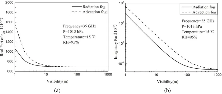
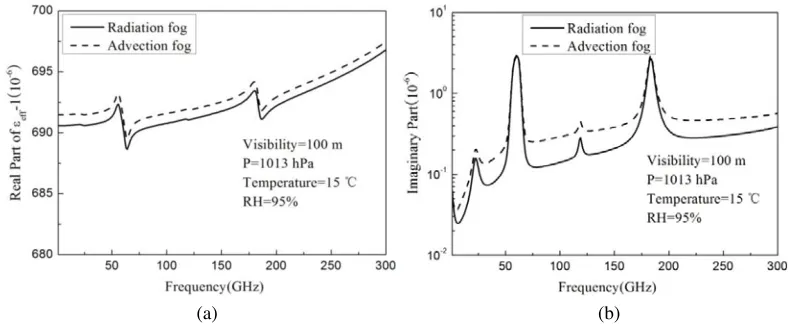
According to the visibility, the liquid water content of fog can therefore be calculated from visibility. We can have the effective permittivity of the fog medium based on formula (10). Figure 1 and Figure 2 show the variations of the relative effective permittivity of fog medium with visibility and frequencies, respectively. We observe from Figure 1 that the effective permittivity decreases with visibility and approaches the values of atmospheric gases when the visibility becomes small enough. Because the size of fog drops is larger, the effective permittivity of advection fog is larger than that of radiation fog with the same visibility. From Figure 2 we can see that the real part of the effective permittivity is not sensitive to the frequency of radio wave. But the imaginary part increases with frequencies and indicates four peaks caused by the absorption of atmospheric gases.

(a) (b)

(a) (b)

Figure 2. Variations of the relative effective permittivity of fog medium with frequencies: (a) real part of ε_eff-1; (b) imaginary part.

3.3. The Effective Permittivity of Rain Medium

Rain medium is formed by rain drops with different shapes and sizes in atmosphere. The diameter of the rain drops ranges from 0.1 to 8 mm, since the drops with diameter larger than 8 mm are unstable and break up. The shape of the rain drop can be assumed to be spherical if its diameter is smaller than about 1.5–2 mm; otherwise, it is oblate ellipsoidal. So, the effective permittivity of rain medium can be calculated by the following formula [13]:

ε_eff =

i=x,y,z

⎛ ⎝ε0+

Dmax

Dmin

N(D)α(D) ε0

ε0−Liα(D) dD

⎞

⎠ u_iu_i. (12)

where ε0 is the permittivity of the atmosphere,which can be obtained from formula (9); N(D) is the raindrop spectrum, which is chosen as Marshall-Palmer-spectrum in this paper; D is the equivalent diameter of a single rain drop;αis the polarization rate;L_i is the diagonal depolarization dyadic, which is determined by the shape of rain drop and L_i = 1₃ for the spherical rain drops; u_i is the direction of axis of rain drop. The polarization rateα is given by [13]

α= v0ε0(εw −ε0) ε0+Li(εw−ε0)

(13)

wherev0 is the volume of one rain drop. For high-frequency fields, the raindrops will reradiate as their dimensions become comparable to the wavelength. Therefore, the polarization rate is modified as

α_h= αl

1 +i(f /f_r)m (14)

whereα_h andα_lare the polarization rates at high and low frequencies, respectively. The characteristic frequencyf_r and value of mare given by [20]. Because the diameters of the rain drops are comparable to the wavelength, high frequency approximation method should be used at millimeter wavelengths.

Figure 3 shows the relations between the relative effective permittivity of rain medium and frequencies for horizontally and vertically polarized waves. We observe that the effective permittivity of the horizontal polarization wave is larger than that of the vertical one. Like fog medium, the real part is also not sensitive to the frequency. And the imaginary part shows two peaks at two frequencies caused by the absorption of atmospheric gases.

4. THE PE METHOD IN MIXED ENVIRONMENTS

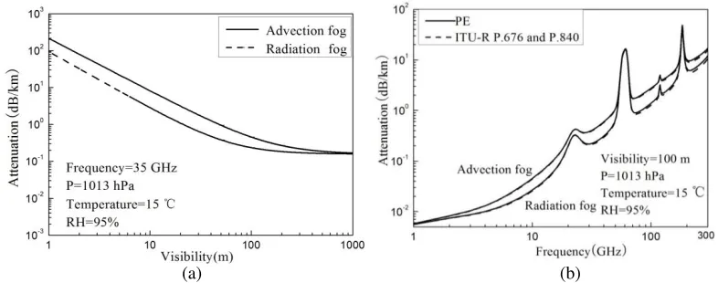
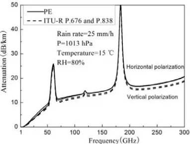
of attenuation in fog environment and rain environment obtained by the PE method are shown in Figure 4 and Figure 5, respectively. For comparison, the corresponding results computed by the ITU-R model are also shown in Figure 4(b) and Figure 5. In fog environment, the attenuation caused by atmospheric gases and fog drops are obtained by ITU-RP.676 and P.840 model, respectively, which can be seen in Figure 4(b). In rain environment, the attenuation caused by atmospheric gases and rain drops is obtained using both ITU-RP.676 and P.838 models, which can be seen in Figure 5. We observe that the results from the two methods are in agreement at millimeter wave band, which demonstrates the validity of the PE method for modeling the attenuation caused by atmospheric gases and hydrometeors. We can also observe clearly that the attenuation in fog environment decreases with visibility. Attenuation in both fog environment and rain environments increases with frequencies and displays some absorption peaks caused by the absorption of atmospheric gases.

(a) (b)

Figure 3. Effective permittivity of rain medium versus frequencies: (a) real part ofε_eff-1; (b) imaginary part.

(a) (b)

Figure 4. Variations of the attenuation in fog environment with: (a) visibility; (b) frequencies.

Figure 5. Variations of the attenuation in rain environment with frequencies.

Geographical Environments

Radiowave Propagation

Model SSFT-PE

Rain

Atmosphere _EnvironmentsMeteorology

Fog

Effective Permittivity Rough Sea

Surface Irregular

Terrain

Figure 6. The propagation model in complex geographical and meteorological environments based on the PE method.

5. RESULTS AND DISCUSSIONS

We apply the model to simulate the propagation of millimeter wave in complex geographical and meteorological environments. The geometry of the complex environments is shown in Figure 7.

A horizontally polarized Gaussian antenna is located at an altitude of 40 m, with beam width of 2◦ and at frequency of 35 GHz. The complex environments are set as follows. It is assumed to be land region between x = 0 km and 10 km, and sea surface with wind speed of 5 m/s for x >10 km. There are a obstacle and an island defined by the trigonometric functions located at 3∼5 km and 12∼14 km, respectively. The atmospheric pressure is 1013 mb, and temperature is 15◦ in the whole computation region. Forx <7 km, it is standard atmosphere environment, and the surface of the ground is assumed to be medium dry ground. Between x = 7 km and 10 km, the rain rate is R = 12.5 mm/h with RH = 80%, and the surface of the ground is assumed to be wet. There is advection fog environment

(a) (b)

Figure 8. The distribution of PF: (a) in standard atmosphere; (b) in complex meteorological environments.

(a) (b)

(c)

with the visibility of 100 m andRH = 95% over rough the sea surface.

Figure 8 shows the distribution of the propagation factor (PF) in standard atmosphere [Figure 8(a)] and complex meteorological environments [Figure 8(b)]. We can observe clearly that the propagation losses for x >7 km in Figure 8(b) are higher than those in Figure 8(a), which is caused by the rain and fog attenuation. It verifies that the PE method can handle effects of complex geographical environments as well as complex meteorological environments.

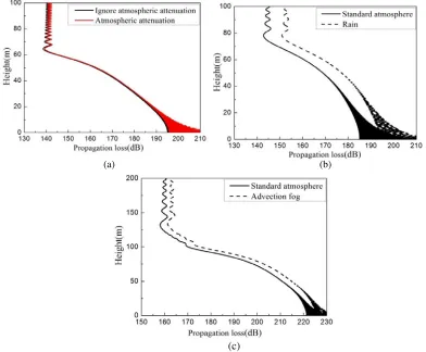
Figure 9 shows the values of propagation loss (PL) versus height at distances of x= 7 km, 10 km and 20 km, respectively. For comparison, the results of ignoring atmospheric attenuation are also shown in Figure 9(a). From the compared results, we observe that the atmospheric attenuation is about 1 dB at x = 7 km. For proving the effects of rain environment, Figure 9(b) gives the propagation losses for two meteorological environments of rain and standard atmospheric environment between x= 7 km and 10 km. Compared with the standard atmospheric environment, the rain attenuation is about 8 dB. Figure 9(c) gives the propagation losses of advection fog and standard atmospheric environment, respectively. From Figure 9(c), we can see that the fog attenuation is about 3 dB lower than the standard.

6. CONCLUSIONS

The study of millimeter-wave propagation in the troposphere is of great significance for practical engineering applications. This work has developed a parabolic equation model for estimating propagation attenuation caused by hydrometeors and atmospheric gases. The model has been employed to simulate the millimeter-wave propagation in complex geographical environments of irregular terrain and rough sea surface, and complex meteorological environments of standard atmosphere, rain and fog. The results demonstrate that the proposed model is suitable for simulating long-range millimeter-wave propagation with complex geographical and meteorological conditions. This scheme will provide an important reference for design and application of millimeter-wave systems. A next step in the research is to study the effect of foliage on millimeter-wave propagation based on PE method.

ACKNOWLEDGMENT

This work was supported by the National Basic Research Program of China (973 Program) under Grant2013CB328904, and the NSAF of China under Grant U1330109.

REFERENCES

1. Sebastian, D., A. Serdal, S. Steffen, M. Hermann, T. Axel, L. Amulf, A. Oliver, Z. Thomas, and K. Ingmar, “A W-band MMIC radar system for remote detection of vital signs,” J. Infrared Milli. Terahz. Waves, Vol. 30, No. 12, 1250–1267, 2012.

2. Ziegler, V., F. Schubert, B. Schulte, A. Giere, R. Koerber, and T. Waanders, “Helicopter near-field obstacle warning system based on low-cost millimeter-wave radar technology,” IEEE Trans. Microw. Theory Tech., Vol. 61, No. 1, 658–665, 2013.

3. Brady, J., N. Behdad, and A. M. Sayeed, “Beamspace MIMO for millimeter-wave communications: System architecture, modeling, analysis, and measurements,” IEEE Trans. Antennas Propag., Vol. 61, No. 7, 3814–3827, 2013.

4. Wang, P., Y. L, and B. Vucetic, “Millimeter wave communications with symmetric uniform circular antenna arrays,”IEEE Commun. Lett., Vol. 18, No. 8, 1307–1310, 2014.

5. Xiong, H., Radiowave Propagation, 487–501, Publishing House of Electronics Industry, Beijing, 2000.

6. Marcus, M. and B. Pattan, “Millimeter wave propagation: Spectrum management implications,” IEEE Microwave Mag., Vol. 6, No. 2, 54–62, 2005.

8. Levy, M. F., Parabolic Equation Methods for Electromagnetic Wave Propagation, IEE Press, London, U.K., 2000.

9. Donohue, D. J. and J. R. Kuttler, “Propagation modeling over terrain using the parabolic wave equation,” IEEE Trans. Antennas Propag., Vol. 48, No. 2, 260–277, 2000.

10. Apaydin, G. and L. Sevgi, “A novel split-step parabolic-equation package for surface-wave propagation prediction along multiple mixed irregular-terrain paths,” IEEE Antennas Propag. Mag., Vol. 52, No. 4, 90–97, 2010.

11. Karimian, A., C. Yardim, P. Gerstoft, W. S. Hodgkiss, and A. E. Barrios, “Multiple grazing angle sea clutter modeling,”IEEE Trans. Antennas Propag., Vol. 60, No. 9, 4408–4417, 2012.

12. Apaydin, G. and L. Sevgi, “MATLAB-based FEM-parabolic-equation tool for path-loss calculations along multi-mixed-terrain paths,”IEEE Antennas Propag. Mag., Vol. 56, No. 3, 221–236, 2014. 13. Sheng, N., C. Liao,W. B. Lin, Q. H. Zhang, and R. J. Bai, “Modeling of millimeter wave propagation

in rain based on parabolic equation method,”IEEE Antennas Wireless Propag. Lett., Vol. 13, 3–6, 2014.

14. Feit, M. D. and J. A. Fleck, “Light propagation in graded-index fibers,” Application Optics, Vol. 17, No. 24, 3990–3998, 1978.

15. Liebe, H. J., “MPM — An atmospheric millimeter-wave propagation model,” Int. J. Infrared Millimeter Waves, Vol. 10, No. 6, 631–650, 1989.

16. Wang, Y. and G. Y. Lu, “Research and stimulation of processing method on radio propagation environment attenuation over the ocean,”Ship Electronic Engineering, Vol. 33, No. 5, 86–89, 2013. 17. ITU-R, “Attenuation by atmospheric gases,” ITU-R Recommendation P.676-9, Geneva, 2012. 18. Sihvola, A. H., Electromagnetic Mixing Formulas and Applications, The Institution of Electrical

Engineers Press, London, 1999.

19. Huang, J. Y., W. He, and S. H. Gong, “The distortion characteristics of a pulse wave propagating through fog medium at millimeter wave band,” J. Infrared Milli. Terahz. Waves, Vol. 28, No. 10, 889–899, 2007.

20. Kharadly, M. M. Z. and S.-V. C. Angela, “A simplified approach to the evaluation of EMW propagation characteristics in rain and melting snow,” IEEE Trans. Antennas Propag., Vol. 36, No. 2, 282–296, 1988.