Adaptive Sharp Boundary Inversion for Transient
Electromagnetic Data
Rui Guo1, 2, Xin Wu1, 2, *, Lihua Liu1, Jutao Li1, Pan Xiao1, 2, and Guangyou Fang1
Abstract—An adaptive sharp boundary inversion scheme is developed to improve resolution with feasibility for transient electromagnetic (TEM) data inversion. By using weighted minimum gradient support (WMGS) constraint, this method focuses the resistivity change areas on layer boundary locations. Prior information describing roughness can be added into the constraint to improve resolution. Furthermore, even though no prior information about layer boundaries is available, it can still reconstruct models with geo-electrical interfaces. Synthetic models prove that this method has a better performance in presenting layer boundaries than smooth-model inversion. Field data of a TEM test line are inverted using this method, which makes the basement layer visualized easily.
1. INTRODUCTION
Transient electromagnetic method (TEM) is a powerful geophysical prospecting tool for mineral, energy and groundwater exploration as well as shallow geological investigation, etc. [1–4]. It is an artificial source electromagnetic detection method based on the process of transmitting the primary electromagnetic impulse to underground and analyzing changes of secondary field versus time to get the electrical characters of the medium [5]. The secondary field is induced by the eddy current underground, typically appearing from 10−6s after the transmitting current is cut off.
Inversion is a major approach for TEM data interpretation, but it is ill-posed because of the non-linearity property of the forward modeling operator [6]. To reduce the chance of stepping into local minima, constraints of spatial resistivity are imposed on optimization functions. The most accepted constraint is the smooth model, assuming the underground resistivity changing continuously. For many years, this constraint has been applied to TEM data inversion in different methods, such as [7– 9]. However, in sedimentary areas, smooth model inversion cannot reflect boundaries of the layers because it produces smooth resistivity transitions. To improve the inversion resolution in sedimentary environments, the visualization of geo-electrical interface is required. Another inversion scheme for reflecting sharp boundary is available [10–12], but it inverts resistivity and layer thickness simultaneously without parameter constraint, which makes the iteration easy to fall into local minima. Unless prior information about layer boundaries is sent into its inversion program, this method is difficult to converge. In this work, weighted minimum gradient support (WMGS) constraint is proposed for TEM sharp boundary inversion. If there is no prior information about layer interface, WMGS constraint degenerates to minimum gradient support (MGS) [13–15] constraint, which can select the minimum volume of area where the gradient of the resistivity is nonzero. By dividing the ground into fixed dense layers, the resistivity with sharp boundary characteristics can be selected adaptively through MGS constraint to match the true resistivity distribution. If prior information about layer interface is available, the
Received 8 March 2017, Accepted 27 April 2017, Scheduled 12 June 2017
* Corresponding author: Xin Wu (wu [email protected]).
proposed weight function adds geological information into inversion, which makes the layer interface to be visualized in a higher resolution.
This paper is organized as follows. In Section 2, the inverse problem models and forward modeling operations are introduced. In Section 3, the scheme of weighted minimum gradient support is explained in detail. In Section 4, the optimization problem is solved. In Sections 5 and 6, synthetic data and filed data inversion are tested to verify this algorithm. Notably, the field test was carried out by CASTEM [16] system. Conclusions follow.
2. WEIGHTED MINIMUM GRADIENT SUPPORT INVERSION
Layered model is applied here. Divide the ground intoN layers with fixed thickness. Taking resolution into consideration, the thickness of theith and (i+1)th layers,tiandti+1, is better to satisfyti/ti+1<1. The resistivity of the ith layer is mi.
The forward modeling operation can be expressed as [4]
Hz = Ia2
∞
0 λ
e−u0|z+h|+
rT Eeu0(z−h)
J0(λr)J1(λa)dλ (1)
where:
(i) Hz is the vertical magnetic field,I the transmitter current strength,athe radius of the transmitter
coil, and r the center offset between the transmitter and receiver coil. z and h are the heights of transmitter and receiver coils.
(ii) rT E is the reflection coefficient noted as rT E = λλ−+ˆuuˆ11, where ˆu1 is calculated from bottom to top
using ˆui =uiuuˆi+1i+ˆu+i+1uitanh(tanh(−−22uuiittii)), and λis the beam of the electromagnetic wave.
(iii) ui is called equivalent beam written asui =
λ2+iωμm
i at theith layer.
Equation (1) can be numerically calculated through fast Hankel transformations [17, 18]. The relation between theoretical datad and resistivity mcan be written as
d=F(m) (2)
whereF is the forward modeling operator shorten for Eq. (1).
In practice, only observed datadobs is available, thus we concern more about the inverse solutionm of Eq. (2). As a property of the ill-posed problem, the inverted parameters with different distributions may have similar field characteristics [19]. To increase the stability of inversion, a reasonable constraint for inversion parameters should be imposed. One of the assumption is that parameters keep continuous in adjacent grids. This constraint is called smooth constraint, widely used in solving inverse problems. However, the continuous resistivity transitions in TEM inversion result in difficulties in distinguishing layer interfaces, hence decreasing the resolution of TEM method.
Minimum gradient support (MGS) is proposed by [13] for reflecting medium’s sharp boundaries, which can be written as
PM GS =
V
∇m· ∇m
∇m· ∇m+βdV (3)
where∇is the gradient operator in the domainV, andβ is a very small positive number called focusing factor. In the 2-norm, Eq. (3) can be transformed to
PM GS =
∇m
√
∇m· ∇m+β 2
2
(4)
For prior information about layer interface to be added, Eq. (4) no longer applies. Weight minimum gradient support (WMGS) function is proposed here, written as
PM GS =
√ ∇m
∇m· ∇m+β0l 2
2
(5)
whereβ0 is a positive number, and lis the weight vector in the format of exponential function.
Suppose that a prior layer interface is located at theNpth layer in the inversion model. Because a
rough weight distribution will cause vibration of inversion results, it is reasonable to define the weight vector l with respect to layer nas
l(n) = 1−αe−γ·|n−Np−N0|(α <1) (6) whereαand γ are used to adjust weight distribution according to prior information, and N0 represents a constant layer number with a typical value of 2∼4. Large gradient appears at N0 layers before low weight occurs. If no prior information is available, α is set to zero. Fig. 1 shows an example of weight distribution. In Fig. 1, suppose that the interface is at 10th layer. Let Np = 2 and choose different
α and γ. If it is known that there is only one interface at the 10th layer, the yellow line is suitable for weighting. If the interface number is uncertain, the red line for weighting is more conservative. However, the blue line without prior information still works, except for some resolution loss. Note that the weight is normalized, henceβ0 needs to be reselected after l changes.
Figure 1. The weight distribution of differentα and γ.
With the constraint of WMGS, the inverse problem can be faced as the solution of the following optimization scheme:
min√ ∇m
∇m· ∇m+β0l 2
2
(7)
s.t. Wd(F(m)−dobs)22< δ (8) where Wd is the data weight, inversely proportional to the noise. Using the regularization method to form the unconstrained optimization function
P =Wd(F(m)−dobs)22+λ√ ∇m
∇m· ∇m+β0l 2
2
(9)
whereλis an ad-hoc parameter [20] defining the total constraint strength.
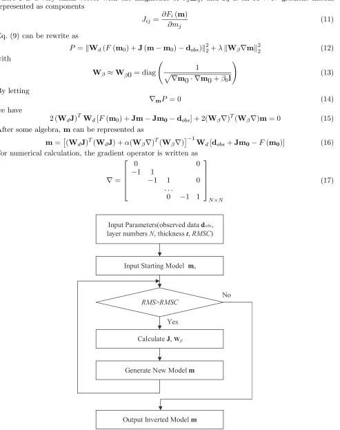
The minimum ofP can be reached when its gradient with respect tomvanishes. The mathematical problem can be solved by an iterative process. Suppose that there is a starting model m0 from which the iteration begins the refinement procedure. IfF is differential atm0 (as we shall always assume that it is), for some sufficiently small vector Δ
where ε is a very small vector with the magnitude of oΔ, and J0 is an M ×N gradient matrix represented as components
Jij = ∂Fi
(m) ∂mj
(11)
Eq. (9) can be rewrite as
P =Wd(F(m0) +J(m−m0)−dobs)22+λWβ∇m22 (12) with
Wβ ≈Wβ0 = diag
1
∇m0· ∇m0 +β0l
(13)
By letting
∇mP = 0 (14)
we have
2 (WdJ)T Wd[F(m0) +Jm−Jm0−dobs] + 2(Wβ∇)T(Wβ∇)m= 0 (15)
After some algebra, mcan be represented as
m= (WdJ)T(WdJ) +α(Wβ∇)T(Wβ∇)−1Wd[dobs+Jm0−F(m0)] (16) For numerical calculation, the gradient operator is written as
∇=
⎡ ⎢ ⎢ ⎢ ⎣
0 0
−1 1
−1 1 0
. . .
0 −1 1 ⎤ ⎥ ⎥ ⎥ ⎦
N×N
(17)
Input Parameters(observed data dobs,
layer numbers N, thickness t,RMSC)
Input Starting Model m0
RMS>RMSC
Calculate J,Wβ
Generate New Model m
Output Inverted Model m
Yes
No
After m is computed, the disagreement between the forward modeling result using m and the real observed data can be measured by
RM S = 1 M V
F(m)−dobs dobs
2
(18)
RM S should be small enough so that the forward modeling result fits observed data well. If it is not the case, m is then considered as the starting approximation of the next iteration. Such procedures keep on until RM S reaches an acceptable level RMSC. During each iteration, λ is selected using a linear searching algorithm to make sure that RM S can be as small as possible.
The inversion procedure can be represented as the flowchart in Fig. 2. In step 3,RMS is calculated by Eq. (18). In step 4, Jand Wβ are calculated by Eqs. (11) and (13). In step 5, the generated model is calculated by Eq. (16). IfRMS is smaller than the level RMSC, the new modelmcan be considered as the inversion result.
3. SYNTHETIC EXAMPLES
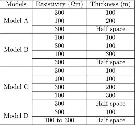
In all the following cases, the synthetic data are simulated by means of Eq. (1) and corrupted with normalized noise with the amplitude of 0.01 nV/Am2. The radius of transmitter coil is 100 m with the current strength 20 A. The receiver is located at the center of transmitter coil. Four models describing different underground structures are generated. Table 1 shows the parameters of these models.
Table 1. Model parameters.
Models Resistivity (Ωm) Thickness (m)
Model A
300 100
100 200
300 Half space
Model B
100 100
300 100
100 300
300 Half space
Model C
300 100
100 100
300 200
100 300
300 Half space
Model D 300 100
100 to 300 Half space
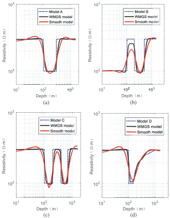
Models A, B and C are layered-models, which have clear interfaces between different layers. In model D, the resistivity increases from 100 Ωm to 300 Ωm gradually, beneath the first sedimentary layer. The responses with noises are presented in Fig. 3, which are used for inversion next. In order to provide high resolution, the ground in the inverse problem is discretized with 39 layers, with the first layer thickness 5 m and increasing ratio 1.09. The targetRMS is set to 2%.
Suppose that no prior information about models A, B and C is available. In model D, prior information is that the interface is located at the 100 m underground, and we use the yellow line presented in Fig. 1 to describe the weight vector. The inversion results of WMGS are compared with that of smooth constraint inversion (see Fig. 4).
( )
Figure 3. Responses of model A, B, C and D, with 0.01 nV/m2/A noises added.
(a) (b)
(c) (d)
lines. Especially in high resistivity areas, WMGS model inversion has better performance than smooth model inversion. In Fig. 4(d), WMGS can reflect both the interface at 100 m and smooth resistivity distribution beneath 100 m. It is shown that the weight (see Fig. 1) selects the model properly.
4. FIELD TEST
The field example is presented here to verify the adaptivity of this algorithm in practice. The test field is in Jianying, Anhui Province, China (see Fig. 5). According to the previous drilled results, there is a quaternary aquifer starting at 60 m underground. The test area is a typical three-layered geological structure. The thickness of the quaternary aquifer is about 400 m. At the bottom is the bed rock layer.
Survey location
Jianying China
(a) (b)
Figure 5. Location of the field test. (a) Survey location in Jianying. (b) Jianying’s location in China.
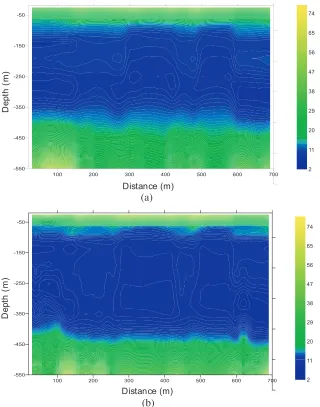
CASTEM system, developed by Institute of Electronics, Chinese Academy of Sciences, was used during the field test. The radius of transmitter coil is 170 m. The transmitting current is 10.8 A with the turned-off time 6µs. More details about the system are shown in Table 2. There are 35 points along a test line. The intervals between two points is 20 m. The observed data after data processing are shown in Fig. 6.
Table 2. Parameters of CASTEM system.
Current 11.3 A
Turn-off time ∼60µs Transmitting frequency 2.5 Hz Effective areas of receiver 1000 m2
Bandwidth of receiver 30 kHz Number of windows 31
First window 90µs Last window 88.881 ms
( )
Figure 6. Observed data received by CASTEM receiver.
Distance (m)
D
ept
h (
m
)
Distance (m)
D
ept
h (
m
)
(a)
(b)
layer at the shallow ground. At the depth of 60 m, the resistivity drops to a low level, which represents the quaternary aquifer. At the bottom is the bed rock. From Fig. 7(a) it is difficult to distinguish the interface of quaternary aquifer layer and basement layer, but Fig. 7(b) can do. It is shown that WMGS inversion has a higher resolution of the layers’ interface than traditional smooth model inversion.
5. CONCLUSION
Traditional TEM inversion for sharp boundaries is easy to step into local minima, hence the smooth model inversion, which is more stable than the former, are widely accepted for data interpretation. However, in sedimentary environments, smooth model inversion has difficulties in reflecting layer interfaces, which results in the resolution loss in TEM data interpretation.
In this work, the weight minimum gradient support constraint is introduced, developed and tested. The weight is selected by a series of exponential functions according to prior information. By solving an optimization problem, the inverted images have large gradient at layer interfaces and become flatter in other areas. This inversion algorithm is tested by synthetic data, which are generated by four different models with noises corrupted. The result shows a better performance than smooth model inversion. At last, a field test is carried out by CASTEM system. After data processing, the inverted model using WMGS shows the interface between quaternary aquifer layer and basement layer with a higher resolution than smooth model inversion.
This method does not need prior information about layer interface but still makes sharp boundaries visualized adaptively. The resolution can be further enhanced by utilizing the proposed weighting scheme. It is especially applicable to inverting data observed in sedimentary areas. For areas with continuous resistivity, it is recommended that smooth model inversion is used, or the focusing factor in WMGS is large.
ACKNOWLEDGMENT
This study is supported by Chinese R&D of Key Instruments and Technologies for Deep Resources Prospecting (the National R&D Projects for Key Scientific Instruments), Grant No. ZDYZ2012-1-03-05 ATEM flight test, data process and interpretation software technology.
REFERENCES
1. He, Z., Z. Zhao, H. Liu, and J. Qin. “TFEM for oil detection: Case studies,” The Leading Edge, Vol. 31, No. 5, 518–521, 2012.
2. Fitterman, D. V. and M. T. Stewart, “Transient electromagnetic sounding for groundwater,”
Geophysics, Vol. 51, No. 4, 995–1005, 1986.
3. Tantum, S. L. and L. M. Collins, “A comparison of algorithms for subsurface target detection and identification using time-domain electromagnetic induction data,” IEEE Transactions on Geoscience and Remote Sensing, Vol. 39, No. 6, 1299–1306, 2001.
4. Nabighian, M., projecteditor, and J. Corbett. “Electromagnetic methods in applied geophysics, Vol. 1: Theory,” SEG, 1988.
5. Rodi, W. and R. L. Mackie, “Nonlinear conjugate gradients algorithm for 2-D magnetotelluric inversion,”Geophysics, Vol. 66, No. 1, 174–187, 2001.
6. Tikhonov, A. N. and V. I. Arsenin, “Solutions of ill-posed problems,”Mathematics of Computation, Vol. 14, Winston, Washington, DC, 1977.
7. Constable, S. C., R. L. Parker, and C. G. Constable, “Occam’s inversion: A practical algorithm for generating smooth models from electromagnetic sounding data,” Geophysics, Vol. 52, No. 3, 289–300, 1987.
9. Vall´ee, M. A. and R. S. Smith, “Application of Occam’s inversion to airborne time-domain electromagnetics,” The Leading Edge, Vol. 28, No. 3, 284–287, 2009.
10. Smith, J. T. and J. R. Booker, “Rapid inversion of two- and three-dimensional magnetotelluric data,” Geophys. Res., 3905–3922, 1991.
11. Marquardt, D. W., “An algorithm for least-squares estimation of nonlinear parameters,” Journal of the Society for Industrial and Applied Mathematics, Vol. 11, No. 2, 431–441, 1963.
12. Auken, E. and A. V. Christiansen, “Layered and laterally constrained 2D inversion of resistivity data,” Geophysics, Vol. 69, No. 3, 752–761, 2004.
13. Portniaguine, O. and M. S. Zhdanov, “Focusing geophysical inversion images,”Geophysics, Vol. 64, No. 3, 874–887, 1999.
14. Zhdanov, M. S., R. Ellis, and S. Mukherjee, “Three-dimensional regularized focusing inversion of gravity gradient tensor component data,”Geophysics, Vol. 69, No. 4, 925–937, 2004.
15. Loke, M. H., I. Acworth, and T. Dahlin, “A comparison of smooth and blocky inversion methods in 2D electrical imaging surveys,” Exploration Geophysics, Vol. 34, No. 3, 182–187, 2003.
16. Wu, X., G. Q. Xue, W. Y. Chen, et al., “Contrast test of the transient electromagnetic system (CASTEM) at the Dawangzhuang iron mine in Anhui province,” Chinese J. Geophys., Vol. 59, No. 12, 4448–4456, 2016, doi: 10.6038/cjg20161207.
17. Anderson, W. L., “A hybrid fast Hankel transform algorithm for electromagnetic modeling,”
Geophysics, Vol. 54, No. 2, 263–266, 1989.
18. Johansen, H. K. and K. Sørensen, “Fast Hankel transforms,” Geophysical Prospecting, Vol. 27, No. 4, 876–901, 1979.
19. Cakoni, F. and D. Colton, Qualitative Methods in Inverse Scattering Theory: An Introduction, Springer Science & Business Media, 2005.