ML Confidential:
Machine Learning on Encrypted Data
Thore Graepel1, Kristin Lauter1, and Michael Naehrig1,2
1
Microsoft Research
{thoreg, klauter, mnaehrig}@microsoft.com
2
Eindhoven University of Technology
Abstract. We demonstrate that, by using a recently proposed leveled homomorphic en-cryption scheme, it is possible to delegate the execution of a machine learning algorithm to a computing service while retaining confidentiality of the training and test data. Since the computational complexity of the homomorphic encryption scheme depends primarily on the number of levels of multiplications to be carried out on the encrypted data, we define a new class of machine learning algorithms in which the algorithm’s predictions, viewed as functions of the input data, can be expressed as polynomials of bounded degree. We pro-pose confidential algorithms for binary classification based on polynomial approximations to least-squares solutions obtained by a small number of gradient descent steps. We present ex-perimental validation of the confidential machine learning pipeline and discuss the trade-offs regarding computational complexity, prediction accuracy and cryptographic security.
1
Introduction
Cloud service providers leverage their large investments in data centers to offer services which help smaller companies cut their costs. But one of the barriers to adoption of cloud services is concern over the privacy and confidentiality of the data being handled by the cloud, and the commercial value of that data or the regulations protecting the handling of sensitive data. In this work we propose a cloud service which provides confidential handling of machine learning tasks for various applications. Machine learning (ML) consists of two stages, the training stage and the classification stage, either or both of which can be outsourced to the cloud. In addition, when both stages are outsourced to the cloud, we propose an intermediate probabilistic verification stage to test and validate the learned model which has been computed by the cloud service. In the protocols we describe here, we identify three parties: the Data Owner, the Cloud Service Provider, and the Content Providers.
When outsourcing computation to a service makes sense, and confidentiality of the data is an issue, then our protocols for providing confidential processing of sensitive data are relevant.
One way to preserve confidentiality of data when outsourcing computation is to encrypt the data before uploading it to the cloud. This may limit the utility of the data, but recent advances in cryptography allow searching on encrypted data and performing operations on encrypted data, allwithout decryptingit. An encryption scheme which allows arbitrary operations on ciphertexts is called a Fully Homomorphic Encryption (FHE) scheme. The first FHE scheme was constructed by Gentry [9], and subsequent schemes [20, 4, 3, 10, 11] have rapidly become more practical, with im-proved performance and parameters. Gentry’s scheme and several of the subsequent FHE schemes have a so-called Somewhat Homomorphic Encryption (SHE) scheme as an underlying building block, and use a technique called bootstrapping to extend it to an FHE scheme. An SHE scheme performs additions and multiplications on encrypted data, but is limited in the amount of such computations it can perform, because encryption involves the addition of small noise terms into ciphertexts. Operating homomorphically on ciphertexts causes the inherent noise terms to grow, and correct decryption is only possible as long as these noise terms do not exceed a certain bound. Noise growth is much larger in homomorphic multiplications than in additions. This means that an SHE scheme can only evaluate polynomial functions of the data up to a bounded degree before the inherent noise grows too large. Bootstrapping, a very costly procedure, is then necessary to reduce the noise to its initial level, enabling fully homomorphic computation. While noise grows exponen-tially in SHE schemes, recent improvements have provided homomorphic schemes in which noise grows only polynomial in the number of levels of multiplications performed [3, 2]. Such schemes are called Leveled Homomorphic Encryption (LHE) schemes, and they allow evaluation of polynomial functions of a higher, bounded degree without resorting to the bootstrapping component.
Recent schemes are based on computational hardness assumptions for problems related to well known lattice problems such as the Shortest Vector Problem (SVP). Specifically, schemes based on the Ring Learning With Errors (RLWE) assumption operate in polynomial rings, where polynomials can alternatively be viewed as vectors in a lattice. It was shown in [16] how the hardness of the RLWE problem is related to SVP.
In practice, as was observed in [14], many useful computational services only require evaluation of low-degree polynomials, so they can be deployed on encrypted data using only an LHE or SHE scheme. In this paper, we propose a confidential protocol for machine learning tasks, called ML Confidential, based on Homomorphic Encryption (HE), and we design confidential machine learning algorithms based on low-degree polynomial versions of classification algorithms. Section 2 describes the general ML Confidential protocol and discusses its security. Section 3 is devoted to explaining basic classification algorithms that can be expressed as low-degree polynomials, including the derivation of division-free, integer (DFI) versions of these algorithms. Section 4 describes the homomorphic encryption scheme we use in our proof-of-concept implementation of the division-free, integer classification algorithms. Our implementation is discussed in Section 5 together with some initial performance numbers and analysis.
Our experiments implement a Linear Means (LM) Classifier and Fisher’s Linear Discriminant (FLD) Classifier on a publicly available data set, the Wisconsin Breast Cancer Data set from [8]. Using up to 100 training and test vectors with up to 30 features each for the training and clas-sification stages, our experiments show that (LM) clasclas-sification can be accomplished in roughly 6 seconds using an unoptimized mathematics software package running on a standard modern laptop. The FLD classifier runs in roughly 20 seconds for vectors with only 10 features. Across all experiments, we observe a slow-down of roughly 6−7 orders of magnitude for operating on encrypted data at these parameter and data sizes. This compares favorably with other recent benchmarks for HE (see [11]).
2
The ML Confidential Protocol and Security Considerations
This section proposes the ML Confidential protocol based on a homomorphic encryption scheme that provides algorithmsHE.Keygen,HE.Enc,HE.Dec, andHE.Evalfor key generation, encryption, decryption, and homomorphic function evaluation. The scheme can be either a symmetric, secret key scheme or an asymmetric, public key scheme. It can be a fully-homomorphic scheme, in which case arbitrary machine learning algorithms can be carried out on the encrypted data by evaluating them with HE.Eval. In a more practical case, it can be a somewhat or leveled homomorphic scheme, where the functionHE.Evalcan only evaluate polynomial functions of the input data with a bounded degree comprised of homomorphic additionHE.Addand multiplicationHE.Multon the message space. Therefore, in that case, machine learning algorithms are restricted to algorithms that can be expressed as polynomials with bounded degree. In either case, let ML.Train and ML.Classify be the training and classification algorithms of the machine learning task which can be homomorphically carried out on encrypted data with the functionHE.Eval.
Three types of parties interact in the protocol: the Data Owner, the Cloud Service Provider, and Content Providers. The protocol comprises the following main components.
Key Generation.The Data Owner executes theHE.Keygenalgorithm for either a private key or a public key version of the homomorphic encryption scheme. For the private key version, the Data Owner shares the private encryption key with the Content Providers and they all securely store the key locally. For the public key version, the Data Owner publishes the public key and securely stores the private key locally.
Encryption and Upload of Training Data. Content Providers encrypt confidential, labeled data to upload to the Cloud. For all classes of training vectors, and for all training vectorsx in each class, the Content Providers encryptxand sendHE.Enc(ek,x) to the Cloud Service Provider along with the unencrypted label of the class. Here ek is the encryption key that is known to the Content Providers, i.e. it is equal to the secret key in the symmetric version and to the public key in the asymmetric version of the scheme. Alternatively, the Content Providers may encrypt preprocessed versions of the training set data, e.g. synthetic data such as class sums or class-conditional covariance matrices (i.e. sufficient statistics) for each class of training vectors.
Training. The Cloud Service Provider computes an encrypted Learned Model. Training vec-tors consisting of encrypted, labeled content, HE.Enc(ek,x), are processed by the Cloud Service Provider. This means that the algorithmHE.Evalof the homomorphic encryption scheme evaluates the machine learning training phaseML.Trainhomomorphically on the encrypted training vectors. An encrypted form of the Learned Model is stored by the Cloud Service Provider and can be returned to the Data Owner on request.
Classification.An encryptionHE.Enc(ek,x) of a test vector x, which usually has not been used in the training stage, is sent to the Cloud Service Provider by the Data Owner or the Content Providers. The Cloud Service Provider evaluates the classification phaseML.Classifyof the machine learning task on the encrypted test vector using the encrypted learned model, and encrypted classifications are returned to the Data Owner. The Data Owner decrypts the results to obtain the classifications.
Verification of the Learned Model.The Data Owner probabilistically tests the Learned Model. The Data Owner encrypts test vectors with known classifications and sends the ciphertexts to the Cloud Service Provider. The Cloud Service Provider classifies the encrypted vectors homomorphi-cally and returns encrypted classification results to the Data Owner. The Data Owner decrypts the results and compares with the known classification labels to assess the test error of the Learned Model in the Cloud.
A MaliciousCloud is a much stronger adversary, who would potentially mishandle calculations, delete data, refuse to return results, collude with other parties, etc. In most of these malicious behaviors, the Cloud would be likely to get caught, and thus damage its reputation if trying to run a successful business.
The verification step we propose is analogous to a naive version of Proof-of-Storage (PoS) protocols. Verification requires the Data Owner to store a certain number of labeled samples locally in order to be able to test correctness (and determine test errors) of the Cloud’s computations. After the training stage, the Data Owner encrypts the test vectors and queries the cloud to provide encrypted classifications of the test vectors, and then the Data Owner decrypts and compares to the correct label. Since we are assuming an Honest but Curious model for the Cloud, the Data Owner only needs to store enough test vectors to determine the test error of the Cloud (or detect any accidental error). We are also implicitly assuming that the Content Providers do not behave maliciously, and correctly encrypt and upload data.
The Cloud must necessarily learn a certain amount of information in order to provide the functionality required. The Cloud computes an encrypted Learned Model from a collection of en-crypted and labeled training vectors in Stage 1 and provides enen-crypted classifications of enen-crypted test vectors in Stage 2. This includes knowing the number of vectors used in the training phase, and the number of test vectors submitted for classification. In addition, our scheme discloses the number of vectors within each class, and also an upper bound on the entries in the test vectors can be deduced once the parameters for the HE scheme and the number of test vectors are known. The underlying HE schemes are assumed to be randomized and have semantic security against passive adversaries, a property which ensures that an adversary cannot distinguish an encryption of one message from another. The Cloud handles encrypted data and performs HE operations, and in the public key setting, can encrypt messages of its choice. However, the Cloud does not obtain decryptions of the ciphertexts that it handles.
3
Polynomial Machine Learning
As discussed in Section 2, a homomorphic encryption scheme can be used to implement the ML Confidential protocol to run machine learning algorithms on encrypted training and test data. An FHE scheme theoretically supports arbitrary computations and thus imposes no restrictions on the ML algorithms used in the protocol. However, implementing a scheme that is fully homomorphic and does not require fixing a specific bound on the complexity of the computation to be done is very costly due to the necessity of bootstrapping.
Useful and flexible as it may be, a fully homomorphic scheme is rarely necessary for most applications, see for example [14]. Instead, if the computation is simple and of low complexity, it is possible to use an SHE or LHE scheme. This not only avoids the expensive bootstrapping procedure, but might also result in smaller parameters to instantiate the scheme, leading to a more practical instantiation of homomorphic encryption. Vice versa, fixing an SHE or LHE scheme in advance raises the question of which applications are possible under the restrictions imposed by the homomorphic capability of the scheme. In practice, we can assume that an SHE or LHE scheme with fixed parameters can homomorphically evaluate polynomials of a fixed limited degree D in the encrypted elements of the message space. This means it can homomorphically evaluate and still correctly decrypt a product ofD message elements, while a product ofD+ 1 elements can not necessarily be decrypted correctly. This section shows that even when using a scheme that is restricted to evaluating polynomials for which the degree bound D is relatively small, it is still possible to perform meaningful machine learning tasks confidentially.
Definition 1 (Polynomial learning/prediction algorithm). Let A: (Rn× Y)m×Rn → Y
be a learning/prediction algorithm that takes a training sample (Rn × Y)m of size m and a test
inputx∈Rn and returns a prediction y∈ Y. If the function A is at most a polynomial of degree
D in its arguments, then we call the learning/prediction algorithm D-polynomial.
Straightforward implementation of many machine learning algorithms requires operations which are not necessarily represented by a low-degree polynomial, ruling out certain algorithms, namely:
Comparison. A comparison x > y for x, y ∈ R is not D-polynomial, unless the inputs are encrypted bit-wise and a very deep circuit for comparison is implemented. This rules out learning algorithms like the perceptron or the support vector machine because they derive their class labels from thresholding real numbers. It also rules out the k-nearest neighbors classifier, which requires ordering neighbors according to distance, and decision trees, which threshold features at the nodes of the tree.
Division.A divisionx/yforx∈Randy∈R\ {0}is notD-polynomial. This rules out algorithms
that rely on matrix inversion such as exact Fisher’s linear discriminant for classification and the standard rule for determining the coefficients in regression.
Other non-polynomial functions.Other functions such as trigonometric functions or the ex-ponential function are not D-polynomial, which rules out methods like exact logistic or probit regression and non-linear neural networks which rely on the evaluation of sigmoidal functions, in particular bounded sigmoid functions which are hard to approximate with polynomials.
Given the restrictions imposed by a homomorphic encryption scheme that can only guarantee correct evaluation of polynomial functions of bounded degree, we are still able to design non-trivial machine learning algorithms. Often, it is even possible to sufficiently approximate the above mentioned functions by polynomials of a bounded degree, for example by means of truncated Taylor series. The exponential function can be approximated by a truncation of its Taylor series, so approximate versions of logistic regression can be implemented with HE as was suggested in [14]. The above definition can be applied directly to regression learning algorithms whereY =Rn0, and tells us that exact least-squares linear regression is not D-polynomial due to the required matrix inversion. Note that classification algorithms cannot beD-polynomial by definition because they have discrete outputs y ∈ Y. However, in this case we can still use the above definition as guidance if we decompose a classification algorithm asA=g◦f, with a mappingf : (Rn× Y)m×
Rn → Rn
0
to a vector of real-valued scores, and a discretization operation g : Rn0 → Y. This decomposition is possible for a large class of algorithms including Linear Discriminant Analysis and Support Vector Machines, and allows the Cloud Service to evaluate the functionf under D -polynomial HE, and the Data Provider to evaluate the functiong. In the following, we focus on the task of binary classification to deduce examples ofD-polynomial machine learning algorithms, but note that tasks like regression and dimensionality reduction could be cast in a similar framework.
3.1 Classification
Let us consider the case of binary classification with inputs in Rn and binary target outputs
fromY ={+1,−1}. We consider a linear classifier of the formA(x;w, c) := sign(f(x;w, c)) with the score function f(x;w, c) :=wTx−c. We assume in the Confidential ML protocol that it is known for two encrypted training examples, whether they are labeled with the same classification (without revealing which one it is). We therefore consider the cardinalities of the positive and negative training sets to be known as well as which ciphertexts encrypt data vectors that belong to the same class. Hence we can carry out operations on these two sets separately. This leads us to consider the simple Linear Means and Fisher’s Linear Discriminant classifiers, both of which require only class-conditional statistics to be evaluated.
Linear Means Classifier. The Linear Means (LM) classifier determines w and c such that
Let Iy :={i ∈ {1, . . . , m}|yi =y} be the index set of training examples with label y and let
my :=kIyk. Calculate the class-conditional mean vectors as my :=my−1sy with sy :=Pi∈Iyxi,
from which we obtain the weight vector as the difference vector between the two class-conditional meansw∗:=m+1−m−1. The value of the thresholdcis calculated using the conditionw∗Tx0−c= 0 for the mid-point, x0 := (m+1+m−1)/2, between the two class means, which gives for the threshold:c∗= (m+1−m−1)T(m+1+m−1)/2. For a given test examplexthe scoref∗(x;w∗, c∗) :=
w∗Tx−c∗ is a quadratic function in the training data and a linear function in the test example and the LM classifier is hence 2-polynomial.
Fisher’s Linear Discriminant Classifier.Now let us move on to a more demanding example, Fisher’s linear discriminant (FLD) classifier [7]. This algorithm is similar to the Linear Means clas-sifier, but does take into account the class-conditional covariances. It aims at finding a projection that maximizes the separation between classes as the ratioS between the varianceσ2
inter between classes and the varianceσ2
intra within classes,
S:= σ 2 inter
σ2 intra
=w TDw
wTCw (1)
withD:=ddT andd:=m
+1−m−1andC:=C+1+C−1. Here,Cy:= m1y Pi∈Iy(xi−my)(xi− my)T is the class-conditional covariance matrix of the data. Taking the gradient w.r.t. w and setting it to zero shows thatw∗ is the solution of a generalized eigenvalue problemDw=λCw. Since D = ddT has rank one, we can write Dw = ad for some a ∈
R and hence Cw∗ ∝ d. Determining w∗ requires solving a linear system of equations, i.e. it can be determined by calculating the inverseC−1 exactly. This requires division, which is not D-polynomial. In what follows, we refer to this approach as the exact FLD algorithm.
In a second approach, we aim at solving the linear system approximately using a least-squares approach so as to obtain a D-polynomial learning/prediction algorithm. The straight-forward cost function isE(w) := 12||Cw−d||2, but instead of the standard Euclidean norm, we choose
||v||2 :=vTC−1v for better conditioning. Then the gradient is∇
wE(w) =Cw−dand we can use gradient descent to find the solutionw∗. Oncewhas been found the threshold can be chosen asc∗:=w∗T(m
+1+m−1)/2.
The challenge then is to approximately solve a linear system using as few multiplications as possible. For the sake of illustration, let us consider standard gradient descent with a fixed learning rateη. If we defineR:=I−ηCanda:=ηd, we obtain the well-known recursionwj+1=Rwj+a. Definingw0=0, we can express the rth order approximationwr ofw∗ as
wr:=
r−1 X
j=0
Rj
a=η
r−1 X
j=0
(I−ηC)j
d. (2)
This series converges if the spectral radius ofR is less than one, i.e., if the absolute value of its largest eigenvalue is less than one, which can be ensured by choosingηsufficiently small. Depending on the order of approximationr, we obtain aD-polynomial FLD algorithm withD= 2(r−1) + 1. Note that the sufficient statistics for the FLD algorithm are the class-conditional means my and covariance matricesCy. If it is desired to reduce the required communication overhead at the cost of increasing the Data Provider workload, then instead of transmitting the raw training data to the Cloud Provider, the Data Provider can calculate and transmit the sufficient statistics for the training data instead.
3.2 Division-Free Integer Algorithms for Classification
be assumed that integers up to a certain size can be embedded into the scheme’s message space, and that the homomorphic operations correspond to the same operations on integers, respectively. In such a setting, it is not possible to perform non-polynomial operations, leaving only polynomial functions on integers as the only practical possibility. To encode a real number by an integer, it can first be approximated to a certain precision by a rational number. Multiplying all such approxi-mations through with a fixed denominator and rounding to the nearest integer provides an integer approximation to the original real numbers. We assume from now on that approximations to real numbers are represented by integers and that we homomorphically embed such representations into the message space of the HE scheme.
In particular, this means that we must avoid divisions since there is no corresponding operation for encoded integers. Below, we describe division-free integer (DFI) versions of the LM classifier and the FLD classifier described in Section 3. The DFI versions of these algorithms are obtained by multiplying with all possible denominators occurring in the computations and adjusting the formulas to exactly compute multiples with the same sign of all magnitudes involved. In detail, computations for both classifiers are as follows.
Linear Means Classifier. For the LM Classifier we compute m−1s+1 and m+1s−1 instead of
m+1 andm−1, and replace the weight vector by
˜
w∗:=m−1s+1−m+1s−1=m+1m−1(m+1−m−1) =m+1m−1w∗. (3)
Similarly, the threshold is replaced by ˜c∗ = 2m2
+1m2−1c∗ using ˜x0 := m−1s+1 +m+1s−1 = 2m+1m−1x0. Given a test vector x, we use the classifier ˜f∗(x; ˜w∗,c˜∗) := 2m+1m−1w˜∗Tx−˜c∗, which simply computes a multiple of the original LM score functionf∗(x;w∗, c∗) with the same sign. The algorithm can be made confidential by encoding all real vector coefficients as integers (as described above). Then one encrypts the input vectors coefficient-wise and carries out the linear algebra operations with vectors of ciphertexts using HE.Add andHE.Mult. Note, that the server only returns the result of the score function for each test example, and that the client takes the sign to obtain the class label, because we assume that our HE scheme does not enable comparison.
Fisher’s Linear Discriminant Classifier. A similar procedure is done for the approximate version of the FLD classifier using gradient descent. We use the same classifying function ˜f∗as for the LM classifier, but with a different weight vector ˜w∗. As above, to avoid divisions, we compute multiples of the class-conditional covariance matrices as ˜C+1=m3+1C+1and ˜C−1=m3−1C−1. In general, we compute ˜C=m3+1C˜−1+m3−1C˜+1=m3+1m
3
−1C, but whenever we can use equal size training classes, i.e.m+1=m−1, we can reduce the coefficients by a factor m3+1.
The gradient descent iteration is done with fixed step size η. When η < 1, we also have to multiply through by its inverse to avoid divisions, which means we need to choose it such that
η−1 ∈
Z. Taking good care of all denominators that need to be multiplied by, we can deduce
that the division free integer gradient descent computes the r-th weight vector ˜wr, which is ˜
wr = (m3+1m3−1η−1)rwr, where wr is the result of the r-th iteration described in Section 3.1. In this way, the DFI version computes multiples of the exact same magnitudes as in the standard gradient descent approach described earlier, resulting in the score function being a multiple of the original score function.
3.3 Other Machine Learning Tasks and Generalization Properties
While we focus on binary classification in this paper, it is certainly possible to extend our methodol-ogy to other machine learning tasks including regression, dimensionality reduction, and clustering. In particular, the case of multivariate linear regression is quite similar to FLD in that the exact so-lution requires a matrix inverse, which can be approximated using gradient descent. Also, principal component analysis (PCA) [12], which is probably the most popular method for dimensionality reduction, can be expressed as a least squares problem the solution of which can be approximated by gradient descent. Clustering may well be the most difficult task in this context, but it would appear that spectral clustering solutions [17] could be approximated in a similar way.
same with respect to the exact algorithm, the restrictions imposed byD-polynomial HE require us to produce predictions which are polynomials of limited degree in the input data. As a consequence, the set of hypotheses that can be reached by aD-polynomial learning algorithm is very limited. One would expect that this limited capacity would have a positive effect on the generalization ability. While we do not have any formal results on this, we believe it may be possible to formalize this idea based on the stability bounds on the generalization error in [18], because the approximations required by SHE can be viewed as a specific form of “early stopping”.
4
A Homomorphic Encryption Scheme
In this section, we describe a homomorphic public-key encryption scheme based on the Ring Learning With Errors (RLWE) problem [16]. It can be used to realize low degree confidential machine learning algorithms as described in Section 3. It extends the encryption scheme in [16] and resembles the LHE scheme from [2] in the RLWE case, as recently described in [6].
For simplicity and later reference in the description of our experiments, we discuss a special case of the scheme, for more details see [16, 2, 6]. Ciphertexts consist of polynomials in the ring
R = Z[x]/(f(x)), where f(x) = xd+ 1 and d = 2k, i.e. integer polynomials of degree at most
d−1. Note that f is the 2d-th cyclotomic polynomial. Computations in R are done by the usual polynomial addition and multiplication with results reduced modulof(x). We fix an integer modulusq >1 and denote by Rq the set of polynomials inR with coefficients in (−q/2, q/2]. For
z∈Z denote by [z]q the unique integer in (−q/2, q/2] with [z]q ≡z (mod q). The message space is the setRtfor another integer modulust >1 (t < q). We use the same notation withqreplaced byt. Thus, messages to be encrypted under the SHE scheme are polynomials of degree at most
d−1 with integer coefficients in (−t/2, t/2]. Let∆=bq/tcbe the largest integer less than or equal to q/t. When applied to a polynomialg ∈R,bgcmeans rounding down coefficient-wise. We also use the notationb·e for rounding to the nearest integer. As error distribution we take the discrete Gaussian distribution χ =DZd,σ with standard deviation σ over R. The parameters d, q, tand
σneed to be chosen in a way to guarantee correctness, i.e. such that decryption works correctly, and security. Section 5 below gives such concrete parameters. Given the above setting (following notation in [6]), we now describe the SHE scheme with algorithms for key generation, encryption, addition, multiplication, and decryption.
SH.Keygen. The key generation algorithm samples s ← χ and sets the secret key sk := s. It samples a uniformly random ring elementa1←Rq and an error e←χand computes the public key pk:= (a0= [−(a1s+e)]q, a1).
SH.Enc(pk, m). Given the public keypk= (a0, a1) and a messagem∈Rt, encryption samples
u←χ, andf, g←χ, and computes the ciphertextct= (c0, c1) := ([a0·u+g+∆·m]q,[a1·u+f]q).
Note that a homomorphic multiplication (as described below) increases the length of a cipher-text. Using relinearization techniques, it can be reduced to a two-element ciphertext again (see e.g. [14, 6]). For the purpose of this paper, we do not consider relinearization, thus ciphertexts can have more than two elements and we describe decryption and homomorphic operations for general ciphertexts.
SH.Dec(sk,ct= (c0, c1, . . . , ck)).Decryption computes [bt·[c0+sk·c1+. . .+skk·ck]q/qe]t.
In general, the homomorphic operations SH.Add and SH.Mult get as input two ciphertexts ct= (c0, c1, . . . , ck) andct0 = (c00, c01, . . . , c0l), where w.l.o.g.k≥l. The output ofSH.Add contains
k+ 1 ring elements, whereas the output ofSH.Multcontainsk+l+ 1 ring elements.
SH.Add(pk,ct0,ct1).Letct1= (c0, c1, . . . , ck) andct2= (d0, d1, . . . , dl). Homomorphic addition is done by component-wise additionctadd= (c0+d0, c1+d1, . . . , cl+dl, cl+1, . . . , ck).
SH.Mult(pk,ct0,ct1). Let ct1= (c0, c1, . . . , ck), ct2= (d0, d1, . . . , dl) and consider the polyno-mialsct1(X) =c0+c1X+. . .+ckXkandct2(X) =d0+d1X+. . .+dlXloverR. The homomorphic multiplication algorithm computes the polynomial product
in the polynomial ringR[X] overR. The output ciphertext isctmlt = (bt·e0/qe, . . . ,bt·ek+l+1/qe).
This scheme has been recently described and analysed in [6] and is closely related to the scheme in [4] and [14]. We refer to these papers for correctness and security under the RLWE assumption. However note that the evaluation of the ciphertext polynomial at the secret key (as computed during decryption) can be written as [ct(sk)]q = [∆·m+v]q, wherev is a noise term that grows during homomorphic operations. Only ifvis small enough, the ciphertext still decrypts correctly. How quicklyvgrows with each multiplication and addition determines the capabilities of the SHE scheme. An advantage of the present scheme is that the factor by whichv grows is independent of the input ciphertext noise (see [2, 6]).
Encoding real numbers. In order to do meaningful computations for ML, we would ideally like to do computations on real numbers, i.e. we need to encode real numbers as elements of Rt. Homomorphic operations under HE correspond to polynomial operations in R with coefficients modulot. To reflect addition and multiplication of given numbers by the corresponding polynomial operations, we resort to the method in [14, Section 4] for encoding integers. We first represent a real number by an integer value. Since any real number can be approximated by rational numbers to arbitrary precision, we can fix a desired precision, multiply through by a fixed denominator, and round to the nearest integer.
An integer valuez is encoded as an elementmz∈Rtby using the bits in its binary represen-tation as the coefficients ofmz. This means we use the following encoding function:
encode :Z→Rt, z= sign(z)(zs, zs−1, . . . , z1, z0)27→mz= sign(z)(z0+z1x+. . .+zsxs).
To get back a number encoded in a polynomial, we evaluate it atx= 2. For the polynomial opera-tions inRtto reflect integer addition or multiplication, it is important that no reductions modulot or modulof occur. A multiplication after which a reduction modulof is done does not correspond to integer multiplication of the encoded numbers any more. The same holds for reductions modulo
t. The value t must therefore be large enough that all coefficients of polynomials representing values in the ML algorithm do not grow out of (−t/2, t/2]. Also the initial polynomial degree of encoded integers (i.e. their bit size) must be small enough so that the resulting polynomials after all multiplications still have degree less thand.
5
Proof of Concept and Experimental Results
In this section, we provide experimental results at a small scale to show how confidential machine learning works in principle. Due to the rather high computational cost of HE, we restrict ourselves to binary classification on a standard data set: the Wisconsin Breast Cancer data set with 569 records obtained from [8]. Data vectors in this set have 30 features and whenever we restrict the number of features in our experiments to somen <30, we take the subset of the firstnfeatures.
With our experimental data we attempt to demonstrate the following claims: on small data sets, basic Machine Learning algorithms on encrypted data are practical. We give performance numbers for both Linear Means (LM) classifier and Fisher’s Linear Discriminant (FLD) classifier, varying both the number of features and the number of vectors used in the training stage to estimate how performance and accuracy scales as these parameters vary. We compare timings for these two classifiers on encrypted and unencrypted data, to show the magnitude of the computational cost for operating on encrypted data. For these experiments, wefixthe security parameters of the system, to model the real-world setting where a cloud system deploys an implementation based on parameters chosen to optimize for performance. In addition, we demonstrate the difference in accuracy when using the DFI version of the FLD algorithm using gradient descent instead of the exact linear algebra version that includes a matrix inversion (in the case of LM the DFI version is exact and does not require an approximation).
data, with fixed security parameters (P1), we vary the number of training vectors and the number of features. Section 5.4 gives performance numbers for the FLD classifier on both unencrypted and encrypted data. On encrypted data, with fixed security parameters (P2), we vary the number of training vectors and the number of test vectors. In Section 5.5, on unencrypted data, we compare the accuracy of the models computed with the exact and DFI versions of the FLD algorithm with varying number of steps in the gradient descent approximation.
5.1 Choice of Parameters
In this subsection, we discuss the specific parameters chosen for our implementation. It has been recently shown in [13] that the hardness of the RLWE problem is independent of the form of the modulus. This means that security is not compromised by choosingqwith a special structure. Using a power of 2 forqdramatically speeds up modular reduction when compared to an implementation whereqis prime. Therefore, as in [6] we choose bothqandtto be powers of 2, i.e.∆=bq/tc=q/t
is also a power of 2. We also use the optimization proposed in [6] to choose the secret keysk=s
randomly with binary coefficients in{0,1}.
To determine parameters that guarantee a certain level of security, one has to consider the best known algorithms to attack the scheme. Its security is assessed by the logarithm of the running time of such algorithms. A security level of`bits means that the best known attacks take about 2` basic operations. We chose parameters considered secure under the distinguishing attack in [15], using the method described in [14, Section 5.1] and [6, Section 6]. For the exact details of the security evaluation, we refer to [15, 14, 6]. Security depends on the size of q, σ, andd, and for a given pairq, σ one can determine a lower bound ford.
Additional conditions follow from ensuring correctness of decryption. As long as the inherent noise in ciphertexts is bounded by ∆/2 =q/2t, decryption works correctly. Since homomorphic computations increase the noise level, this bounds the number of computations from above. In the division free integer algorithms the encrypted numbers tend to grow with the number of operations due to multiplications by denominators. To ensure meaningful results,tneeds to be greater than all the coefficients of message polynomials that are held and operated on in encrypted form. The size of the standard deviation for the error terms and the desired number of homomorphic operations bound ∆ and therefore q from below. For our implementation, we determined these quantities experimentally and then chose the degreedaccording to the security requirements.
5.2 Timings for basic HE operations
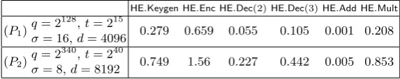
We implemented the HE scheme described in Section 4 and the division-free integer ML algorithms under HE in the computer algebra package Magma [1], using internal functions for polynomial arithmetic and modular reductions. Table 1 summarizes timings for the HE operations. The con-fidential version of the DFI-LM classifier uses the first parameter set (P1) to encode and encrypt data. Parameters (P2) were chosen for encoding and encryption for the confidential version of the 3-step FLD method. Due to its higher complexity and the higher value fort it requires a much larger value forq.
HE.Keygen HE.Enc HE.Dec(2)HE.Dec(3)HE.Add HE.Mult
(P1)q= 2 128
,t= 215
0.279 0.659 0.055 0.105 0.001 0.208
σ= 16,d= 4096
(P2)q= 2
340,t= 240
0.749 1.56 0.227 0.442 0.005 0.853
σ= 8,d= 8192
Table 1.Timing in seconds for HE operations: key generation, encryption, decryption of 2- or 3-element ciphertexts, homomorphic addition and multiplication.
seconds (s). No communication costs are included in these experiments since the computations are all done on one machine. Parameters (P1) have 128 bits of security with distinguishing advantage 2−64. Security for (P
2) is around 80 bits due to smallσcompared toq.
5.3 Linear Means Classifier
For the Linear Means Classifier, the exact and the DFI versions of the algorithm coincide, so there is no difference in the quality of the output. We compare in this section the timings for the encrypted and unencrypted DFI versions of the algorithm. The Linear Means Classifier experiments in this section were run with security parameters (P1),
q= 2128, t= 215, σ= 16, f=X4096+ 1.
The data was preprocessed by shifting the mean to 0 and scaling by the standard deviation. Also, precision of computation was set at 2 digits, which means real numbers are multiplied by 100 and rounded to integers.
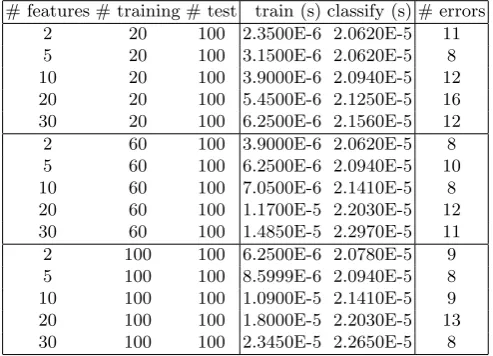
Timings on Unencrypted Data for DFI-LM. Each line in the tables reports the number of features used, the number of training vectors used in the training stage to build the classifier, the number of test vectors used to test the model, the time spent in the training stage, the timeper test vectorto classify, and the number of errors in the classification of test vectors.
# features # training # test train (s) classify (s) # errors 2 20 100 2.3500E-6 2.0620E-5 11
5 20 100 3.1500E-6 2.0620E-5 8
10 20 100 3.9000E-6 2.0940E-5 12 20 20 100 5.4500E-6 2.1250E-5 16 30 20 100 6.2500E-6 2.1560E-5 12
2 60 100 3.9000E-6 2.0620E-5 8
5 60 100 6.2500E-6 2.0940E-5 10 10 60 100 7.0500E-6 2.1410E-5 8 20 60 100 1.1700E-5 2.2030E-5 12 30 60 100 1.4850E-5 2.2970E-5 11 2 100 100 6.2500E-6 2.0780E-5 9 5 100 100 8.5999E-6 2.0940E-5 8 10 100 100 1.0900E-5 2.1410E-5 9 20 100 100 1.8000E-5 2.2030E-5 13 30 100 100 2.3450E-5 2.2650E-5 8
Table 2.DFI-LM Unencrypted Data
Remarks.Note that the time for classifying vectors is relatively constant, which is as expected. The number of classsification errors varies, but tends to decrease as the size of the training set increases.
# features # training # test train (s) ee-train (s) classify (s) ee-test (s)
2 20 100 0.095 19.953 0.327 133.843
5 20 100 0.156 50.172 0.899 343.250
10 20 100 0.391 101.141 1.938 708.969
20 20 100 0.831 201.578 3.880 1405.875
30 20 100 1.374 303.937 5.961 2122.719
2 60 100 0.127 59.641 0.325 133.703
5 60 100 0.484 148.125 0.879 337.953
10 60 100 0.996 309.078 1.864 688.531
20 60 100 2.504 601.688 3.841 1400.266
30 60 100 3.346 899.953 5.838 2106.453
2 100 100 0.565 98.938 0.417 143.719
5 100 100 0.835 249.359 0.998 351.078
10 100 100 2.629 499.063 1.971 699.531
20 100 100 4.034 999.156 3.989 1403.172
30 100 100 6.221 1504.297 6.038 2110.000
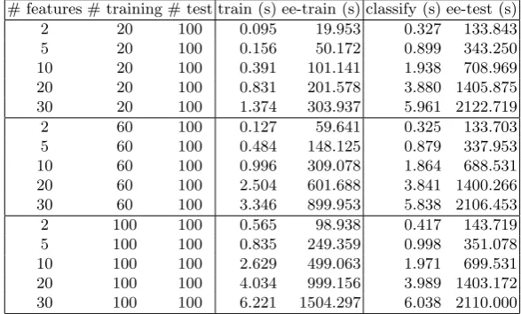
Table 3.DFI-LM Encrypted Data
Remark 5.3
1. The time for classifying a test vector and for encoding and encrypting the test vectors stays relatively constant as the number of training vectors increases, as expected.
2. The time for computing the classifier in the training stage grows roughly linearly with the number of training vectors. This is expected as long as the security parameters are fixed, as is the case here.
3. The time for encoding and encrypting data in the training stage grows roughly linearly with the number of training vectors. Again, this is expected as long as the security parameters are fixed, as we have modeled here.
4. For a fixed training set size, the time for computing the classifier grows approximately linearly with the number of features. Similarly, the time for classifying a test vector, and the time for encoding and encrypting the training and the test vectors each grow approximately linearly with the number of features.
5. The approximate order of magnitude of the slow-down due to operating on encrypted data is 6 or 7 orders of magnitude. This compares favorably with the slow-down for performing an AES encryption operation on encrypted data reported in [11].
6. Note that even with this preliminary unoptimized implementation, both the training stage and the classification of a test vector can be performed on encrypted data in roughly 6 seconds using a Linear Means Classifier on 100 training vectors with 30 attributes.
5.4 Fisher’s Linear Discriminant classifier
The experiments in this section were run with security parameters (P2),
q= 2340, t= 240, σ= 8, f =X8192+ 1.
The data was preprocessed by shifting the mean to 0 and scaling by the standard deviation. Also, precision of computation was set at 2 digits, which means real numbers are multiplied by 100 and rounded to integers. The DFI version of the FLD algorithm was run using 3 steps in the gradient descent method with step sizeη= 0.1.
# features # training # test train (s) classify (s) # errors 2 20 100 2.6600E-4 1.7200E-6 11
5 20 100 7.5000E-4 1.8800E-6 7
10 20 100 2.4690E-3 2.1800E-6 9 20 20 100 9.2030E-3 2.9700E-6 6
30 20 100 0.020390 3.9100E-6 8
2 60 100 4.0700E-4 1.5700E-6 8
5 60 100 1.7030E-3 1.7200E-6 7
10 60 100 6.2190E-3 2.1800E-6 8
20 60 100 0.024125 2.9700E-6 9
30 60 100 0.054250 3.9000E-6 8
2 100 100 5.7800E-4 1.5600E-6 10 5 100 100 2.6410E-3 1.7200E-6 7
10 100 100 0.0100 2.1900E-6 8
20 100 100 0.039282 2.9700E-6 6 30 100 100 0.087594 3.9000E-6 3
Table 4.3-step DFI-FLD Unencrypted Data
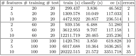
Timings on Encrypted Data for 3-step DFI-FLD. Each line in the table reports the number of features, the number of training vectors used in the training stage to build the classifier, the number of test vectors used to test the model, the time spent in the training stage, the time per test vector to classify, the total time spent on encrypting and encoding the test vectors (in the “ee” column in Table 5), and the number of errors in the classification of test vectors.
# features # training # test train (s) classify (s) ee (s) errors
2 20 20 299.437 3.836 46.562 2
5 20 20 1309.578 10.049 117.033 1
10 20 20 4472.922 20.857 236.514 1
2 60 20 939.156 6.488 51.280 1
5 60 20 3612.953 9.707 117.158 1
10 60 20 12211.719 20.465 235.236 1
2 100 100 1420.781 3.850 619.828 10
5 100 100 6017.688 10.364 1636.265 8 10 100 100 20222.515 21.572 3351.718 35
Table 5.3-step DFI-FLD Encrypted Data
Remark 5.4
1. The timings in the last line for 10 features and 100 training vectors should be disregarded, be-cause the 35 classification errors indicate that the computation exceeded the allowable bounds for the amount of computation which could be correctly done with these security parameter sizes. This computation most likely resulted in decryption errors and should be redone with larger system parameters.
2. Note that for both the LM and the FLD algorithms, the time spent in computing on encrypted vectors is dominated by the time spent to encrypt the data. That is due to the fact that each entry to be encrypted requires a multiplication of two polynomials of degreed, wheredis either 4096 or 8192 in these experiments. Although Magma does have fast multiplication techniques implemented, this is an aspect of the system where performance can be significantly improved in a robust high-performance implementation.
4. The time spent in the training stage grows roughly linearly with the number of training vectors. Also the time spent on encoding and encryption grows linearly with the number of features. 5. Time spent on classifying test vectors is relatively constant as the number of training vectors
increases, as expected.
6. The time spent on classifying test vectors grows roughly linearly with the number of features. 7. As for the confidential LM algorithms, we observe a slow-down of roughly 6−7 orders of
magnitude when executing the 3-step DFI-FLD algorithm on encrypted data under HE. 8. Despite the significant performance penalty for operating on encrypted data, note that
clas-sification of test vectors with 10 features is accomplished in 20 seconds with an unoptimized implementation of HE. This time is relatively independent of the number of training vectors used in the training stage for fixed system parameters. However, it is dependent on the amount and size of the data to be processed in the sense that the system parameter sizes must be in-creased once the bounds on the amount of computation which can be properly handled for a given parameter size are exceeded.
5.5 Comparing the accuracy of exact and DFI versions of gradient descent
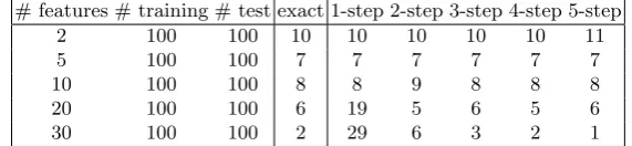
In Section 5.4 above, we gave performance numbers for the DFI version of the gradient descent method for Fisher’s Linear Discriminant Classifier. The gradient descent method for minimizing the cost function is an approximation algorithm, whereas there is an exact algorithm for minimiz-ing the cost function which requires matrix inversion. In this section, we compare the accuracy of the models obtained when using the exact version of FLD versus using the gradient descent approximation method with a varying number of steps. In Table 6 we give the number of classifi-cation errors for the exact version of FLD and the gradient descent method with 1−5 steps. These experiments were performed on unencrypted data, with step sizeη= 0.1. Based on these results, three steps seemed to be sufficient in the gradient descent method for these data set sizes, so we used 3 steps in all experiments in Section 5.4 to produce encrypted and unencrypted timings for FLD.
# features # training # test exact 1-step 2-step 3-step 4-step 5-step
2 100 100 10 10 10 10 10 11
5 100 100 7 7 7 7 7 7
10 100 100 8 8 9 8 8 8
20 100 100 6 19 5 6 5 6
30 100 100 2 29 6 3 2 1
Table 6.# errors in exact and DFI-FLD classification on unencrypted data
6
Conclusions and Future Work
With advances in machine learning and cloud computing the enormous value of data for commerce, society, and people’s personal lives is becoming more and more evident. In order to realize this value it will be crucial to make data available for analysis while at the same time protect it from unwanted access. In this paper, we pointed out a way to reconcile these two conflicting goals: Confidential Machine Learning. We formalize the problem in terms of a multi-party data machine learning scenario involving a Data Owner, Data Providers, and a Cloud Service Provider and describe the desired functionality and security properties. We showed that it is possible to implement Confidential ML based on a recently proposed Homomorphic Encryption scheme, using polynomial approximations to known ML algorithms.
polynomial machine learning algorithms implementing non-linear mappings. Other open problems include the question, which protocols will be useful in practical data analysis scenarios, and how the computational burden can be optimally distributed between cloud and client taking into account the cost of communication. Furthermore, one can imagine even more complex multi-party scenarios in which multiple data-owners (e.g., Amazon, Netflix, Google, Facebook) would like to provide inputs for a single machine learning problem (e.g., product recommendation) without disclosing their data.
References
1. Wieb Bosma, John Cannon, and Catherine Playoust. The Magma algebra system. I. The user language.
J. Symbolic Comput., 24(3-4):235–265, 1997. Computational algebra and number theory (London, 1993).
2. Zvika Brakerski. Fully homomorphic encryption without modulus switching from classical GapSVP. InAdvances in Cryptology - Crypto 2012, volume 7417 ofLecture Notes in Computer Science, pages 868–886. Springer, 2012.
3. Zvika Brakerski, Craig Gentry, and Vinod Vaikuntanathan. (Leveled) fully homomorphic encryption without bootstrapping. In Shafi Goldwasser, editor, Innovations in Theoretical Computer Science – ITCS 2012, pages 309–325. ACM, 2012.
4. Zvika Brakerski and Vinod Vaikuntanathan. Fully homomorphic encryption from Ring-LWE and security for key dependent messages. In Phillip Rogaway, editor,CRYPTO, volume 6841 ofLecture Notes in Computer Science, pages 505–524. Springer, 2011.
5. R. O. Duda, P. E. Hart, and D. G. Stork. Pattern Classification. John Wiley and Sons, 2nd edition, 2000.
6. Junfeng Fan and Frederik Vercauteren. Somewhat practical fully homomorphic encryption. Cryptology ePrint Archive, Report 2012/144, 2012. http://eprint.iacr.org/.
7. R. A. Fisher. The use of multiple measurements in taxonomic problems.Annual Eugenics, 7(2):179– 188, 1936.
8. A. Frank and A. Asuncion. UCI machine learning repository,http://archive.ics.uci.edu/ml, 2010. 9. Craig Gentry. Fully homomorphic encryption using ideal lattices. In Michael Mitzenmacher, editor,
STOC, pages 169–178. ACM, 2009.
10. Craig Gentry, Shai Halevi, and Nigel Smart. Better bootstrapping in fully homomorphic encryption. InPublic Key Cryptography - PKC 2012, volume 7293 ofLecture Notes in Computer Science, pages 1–16. Springer, May 2012.
11. Craig Gentry, Shai Halevi, and Nigel P. Smart. Homomorphic evaluation of the AES circuit. In
Advances in Cryptology - Crypto 2012, volume 7417 of Lecture Notes in Computer Science, pages 850–867. Springer, 2012.
12. I.T. Jolliffe. Principal Component Analysis. Springer Verlag, 1986.
13. Adeline Langlois and Damien Stehl´e. Hardness of decision (R)LWE for any modulus. Cryptology ePrint Archive, Report 2012/091, 2012. http://eprint.iacr.org/.
14. Kristin Lauter, Michael Naehrig, and Vinod Vaikuntanathan. Can homomorphic encryption be practi-cal? InProceedings of the 3rd ACM Cloud Computing Security Workshop, CCSW ’11, pages 113–124, New York, NY, USA, 2011. ACM.
15. Richard Lindner and Chris Peikert. Better key sizes (and attacks) for LWE-based encryption. In Aggelos Kiayias, editor,CT-RSA, volume 6558 ofLecture Notes in Computer Science, pages 319–339. Springer, 2011.
16. Vadim Lyubashevsky, Chris Peikert, and Oded Regev. On ideal lattices and learning with errors over rings. In Henri Gilbert, editor,EUROCRYPT, volume 6110 of Lecture Notes in Computer Science, pages 1–23. Springer, 2010. Full version available athttp://eprint.iacr.org/2012/230.
17. Andrew Y. Ng, Michael I. Jordan, and Yair Weiss. On spectral clustering: Analysis and an algorithm. InAdvances in Neural Information Processing Systems 14, pages 849–856. MIT Press, 2002.
18. Tomaso Poggio, Ryan Rifkin, Sayan Mukherjee, and Partha Niyogi. General conditions for predictivity in learning theory. Nature, 428:419–422, 2004.
19. Ronald L. Rivest. Cryptography and machine learning. In Advances in Cryptology - ASIACRYPT 91, pages 427–439. Springer, 1993.
20. Nigel P. Smart and Frederik Vercauteren. Fully homomorphic encryption with relatively small key and ciphertext sizes. In Phong Q. Nguyen and David Pointcheval, editors,Public Key Cryptography, volume 6056 ofLecture Notes in Computer Science, pages 420–443. Springer, 2010.