Channel Estimation Based On Compressive Sensing In Ofdm Systems

Channel Estimation Based on Compressive Sensing in OFDM

Systems

YuanHang Liu*, ZongGang Ye*, Shuai Peng*

*Chongqing Key Lab of Mobile Communications Technology, Chongqing University of Posts and Telecommunications, Chongqing 400065, P. R. China

Abstract

In OFDM systems, channel estimation is absolutely necessary for receiver design. Applying the theory of

compresssive sensing to channel estimation in OFDM systems can not only reduce the number of the using

pilots, but also improve the performance of channel estimation. an improved generalized orthogonal matching pursuit algorithm (IGOMP) is proposed for

channel estimation due to the low accuracy of channel estimation in the generalized orthogonal matching pursuit (GOMP) algorithm, the time of channel

estimation in the orthogonal matching pursuit (OMP) algorithm is long, and all need a priori information

with channel sparseness. The proposed algorithm which is used for channel estimation bring in a filtering mechanism to ensure the correctness of the currently

selected atoms, to determine the step size based on the variation of the residual value, and to use the noise

power to ensure the iteration stop threshold. Simulation results show that the proposed algorithm has a good channel estimation performance without

prior information of the sparsity with a short computation time, which compared with the least

square algorithm, the orthogonal matching pursuit algorithm and the generalized orthogonal matching pursuit algorithm.

Keywords: orthogonal frequency division multiplexing, compressive sensing, channel estimation

1.

Introduction

As a highly effective multi-carrier modulation

solution, OFDM technology has sound performance of

combating frequency selective fading and high bandwidth efficiency[1]_{. It is widely used in wireless communication}

system currently. Channel estimation is a hotspot in the research of communication field, and its quality plays an important role in the property of the whole communication

system[2]. The pilot-assisted channel estimation algorithm in OFDM system is the most commonly used method[3],

therein exists an algorithm called Least Square[4], simple in structure and low in computational complexity, through a way of estimating the channel information from pilot

first and then refactoring the channel information of data sub-carriers through the interpolation method. This

method is applied to the dense channel, but not proper when there is less number of multipath for the channel. Compressive sensing theory shows a new method of signal

acquisition and processing. it sampling the compressible sparse signal in a way of far below the Nyquist rate and

regaining the original signal exactly[5].

With the development and maturity of the compressive sensing technology, it has been used in the OFDM sparse

channel estimation in the field of communication and signal by scholars at home and abroad. Due to the sparsity

characteristic of the wireless channel, which means that the tap coefficient close to zero elements or numerical zero elements is relatively more, the multipath parameters

needed to be estimated is decreased. Instead of getting the channel information on the data subcarrier by the

interpolation method, channel estimation based on compressive sensing can estimate the multipath parameters and reconstruct the information of the channel

via the information from the pilot. By doing this, the expenditure on the pilot is lowered down, therefore it can

system spectrum efficiency effectively. That is the reason why sparse channel estimation algorithm has always been

taken as a search hot point in the field of academic and industry[6]. In the paper [7], the author proposed that applying matching pursuit (MP) algorithm to OFDM

sparse channel estimation. In the paper [8], OFDM sparse channel estimation method based on the orthogonal

matching pursuit (OMP) algorithm was raised. According to literature [9], a generalized orthogonal matching pursuit (GOMP) algorithm is proposed. The GOMP algorithm

selected a few atoms that is the biggest multiplied with residual. OMP algorithm is a special GOMP algorithm. Compared to OMP algorithm, GOMP has a higher

computing speed.

2.

OFDM system model

Binary Information QPSK Modulation S/P Pilots Insertion IFFT CP Insertion P/S Data Receiving QPSK Demodulation Channel Estimation FFT CP Removing P/S S/P Channel Noise

Fig.1 OFDM system model

OFDM system diagram is shown in Figure 1, assuming OFDM system has N subcarriers, among which P subcarriers are used to convey the pilot information. The

1 ×

N dimension signal of the receiving end can be expressed as:

W XFh W

XH

Y = + = + (1)

Whereby, Matrix X of Dimension N×N in

Formula (1) can be expressed as

)) 1 ( ) 3 ( ) 2 ( ) 1 ( ) 0 ( ( −

= X X X X ...X N

X diag , , , , , , and

] [h0,h1,h2,...,hL−1

=

h ;

_h

is the impulse response to

the discrete time-domain of the channel; H is the corresponding frequency domain response;

F

is N×L

dimension matrix; W is the Gaussian white noise of 1

×

N dimension vectors.

When the channel coherence time is far more than the OFDM symbol duration, the channel parameters in one

OFDM symbol can be considered constant, and the channel impulse response can be expressed as:

) ( ) ( 1 0 i L i i t h t

h =

∑

σ −τ −

=

(2)

In formula (2), L is the total number of the tapped delay in the channel model, and hi is the complex gain of Tap i;

the sparsity of the channel is mainly shown in the number of several minority elements with relatively larger values or nonzero elements in [h0,h1,h2,...,hL−1] set; τi is

the delay of Tap i.

Set the selective matrix of P×N dimension as S

through which the N subcarriers will select out the P pilot positions, thus the corresponding signals received

from the receiving end of the P pilot signals can be expressed as: 1 P 1 L L P 1 P 1 L L P P P 1 p W h Α W h F X Y × × × × × × × × + = + = (3)

In formula (3), the formula 1 P

P SXS

X × = − for P×P dimension matrix presents the signals sent from pilot tones; W_P×₁=SW for the P×1 dimension vector presents the noises of the channel;

              = − − − − − − × N c L j N c j N c L j N c j p N p N N N e e e e

N _{2 0 2 ( 1)}

) 1 ( 2 0

2 _{1 1}

1 π π π π     L P

F for the

L

P× dimension matrix is the fast fourier transform (FFT)

matrix at the corresponding P pilot, where N nl j nl e f π 2 − = , SY

YP×1= for the P×1 dimension vector present the

corresponding signals accepted at pilot from the receiving end, and the P×L dimension matrix AP×L=Xp×pFP×L is a

measurement matrix. Besides, YP×1，AP×L are all known

signals for the receiving end. It is a reconstruction problem of sparse signals to recover the h_L×₁ process according to formula (3), which can be resolved by compressive

sensing theory.

3.

An improved generalized orthogonal

matching pursuit algorithm

Generalized orthogonal matching pursuit (GOMP)

algorithm selected a few atoms that is the biggest multiplied with residual in each iteration. Compared with

OMP algorithm, GOMP have a higher running speed and its computation complexity is lower. GOMP algorithm process is as follows:

Input: M×N dimension measurement matrix A , 1

×

N dimension observation vector Y , initialize and each time choose S atoms, The value of the channel sparseness K.

Output: Estimation of the time domain impulse response of the channel _hˆ

(1) Intialize r0 =Y, index value Λ0=

∅

, candidate set ∅

=

0

Α , stage t=1;

(2) Calculate [_AT_{rt 1}] −

=abs

u , equals to calculate

N j≤

≤

−1, j ,1 t a

r , choose S biggest numeric in u, and

collect these values sequence number corresponded to A

into a J0 set.

(3) For Λt =Λt−1∪J0 , update index set j

1 t

t Α a

Α = ₋ ∪ (j ∈J0).

(4) Determine the least square solution of Y=Αth:

h Α y

hˆ=argmin − t ; and update residual error

h Α y

rt = − tˆ.

(5) t=t+1, if t≤min(K,M/S) or rt−1 2 ≤α Where

α

is a small number, return to step (2); if not, stop iterating.

From the steps above it can be seen that GOMP selected a few atoms that is the biggest multiplied with

residual in each iteration, wrong atoms would be chosen in the iteration. Secondly, GOMP algorithm can reconstruct

the signal accurately only if the sparseness of the channel is known in advance, however, the sparse degree always cannot be foreseen in practical condition. According to the

experiment and simulation, GOMP algorithm for channel estimation is not as effective as OMP algorithm.

Therefore, an improved generalized orthogonal matching pursuit (IGOMP) algorithm has been proposed for the characteristics of the GOMP algorithm. Under the

condition of unpredicted sparse degree, IGOMP can estimate channel information accurately and with a low bit error rate.

Compared with the GOMP algorithm, the IGOMP algorithm has the following differences

First, the GOMP algorithm chooses two or more atoms during each iteration, but the selected atoms may not be appropriate, which makes the iterative signal not be able to

approximate the original signal. Thus, at the end of each iteration, a filtering mechanism is introduced by comparing the quadratic norm r₂ of the vector in the current iteration with the quadratic norm rt-1₂ of the

residual vector of the previous iteration. If rt-12≤ r2, it

means that the number of atoms selected this is not enough, it will increase the support set of atoms. Otherwise

iterates.

Secondly, in the GOMP algorithm, when the residual is less than a certain threshold, it indicates that the support

set may already be closer to the support set of the original signal, and the step size needs to be reduced. Therefore, in the improved algorithm, when r₂≤exch∗Y ₂, where exch is the variable step threshold parameter. in this paper, the value of

exch

is 0.3. The support set L

increments by only 1, that is, by the time S is equal to 1 when the secondary norm of the residual is less than a

certain threshold.

Finally, the OMP algorithm and the GOMP algorithm can reconstruct the signal accurately when the sparsity of

the channel is known. However, in the actual environment, the sparseness of the channel is often unpredictable.

Therefore, the reconstruction algorithm of the channel needs to find a suitable threshold for determining whether the iteration should be terminated. If the channel can be

reconstructed accurately, the last remaining residual must satisfy the following conditions:

p p

p− ≤

=

2

2 Y Th

r (4)

Where p represents the power of Gaussian white

p

+

≤α

2

r , where

α

is a small constant.

On this basis, the IGOMP algorithm steps are as

follows ：

Input: M×N dimension measurement matrix

A

, 1

×

N dimension observation vector Y , initialize and choose Satoms.

Output: Estimation of the time domain impulse

response of the channel hˆ

Step 1 ： Intialize residual error r₀ =Y, index value

0

Λ =∅, candidate setΑ0 =∅, initialize support set L=S,

stage t=1;

Step 2: Calculate [_AT_{rt 1}] −

=abs

u , equals to calculate

N j≤

≤

−1, j ,1

t a

r ,Where aj represents the column j

of the measurement matrix

A

. choose L biggest numeric in u , and collect these values sequence number corresponded to A into a J0 set.

Step 3: For Λt=Λt−1∪J0, the number of elements in the index value Λt−1 is P. ΑΛ ={aj}(j∈Λ).

Step 4: Determine the least square solution of Y=Αth:

h Α y

hˆ=argmin − t ; and renewal the residual error

h Α y

rt= − tˆ.

Step 5: If rt-1 ₂≤ r ₂, turn to step 6; if not, turn to step

8.

Step 6: If r2≤exch∗Y2, change the section value, step length, for L=L+1, carry on step 2; if not, turn to step 7.

Step 7: For L=L+S, carry on step 2.

Step 8: Update index set and residual error, Λ

=

Λt ，rt =r，t=t +1 ， Carry on step 9.

Step9: If ≤α+p

2

r , stop iterating, output channel

time impulse response hˆ, Or else, enter the step 2.

4.

Simulation and performance analysis

In order to verify the effectiveness of the proposed

algorithm, the following simulation is taken in this paper, The simulation parameters are as follows in table 1.

Table 1: Simulation parameters

Parameters value

Bandwidth 48kHz

Sub-carrier Number 1024

Cyclic Prefix Length 256

Modulation and Demodulation 4PSK

Maximum Time Delay: 2ms

Maximum Doppler Shift : 1Hz

Channel Sparseness: 2

Channel Length: L 50

Signal-to-Noise Ratio 0-30dB

Simulation Number: m 1000

System simulation uses the bit error rate (BER) and

the normalized mean square error (MSE) as indicators, to make a comparison in the channel estimation performance

differences among the LS algorithm, the OMP algorithm, GOMP algorithm and IGOMP algorithm. The normalized mean square error (MSE) formula is:

2

1 2

1

/

∑

∑

= =

∧

−

= m

i i m

i i

i h h

h

MSE (5)

In the formula, m is the simulation number of times.

i

hˆ stands for the estimated value of the channel impulse response in the

i

simulation experiment. hˆi is the real

value of the channel impulse response in the

i

simulation

experiment.

4.1 A comparison of the performance of MSE and BER

among different algorithms

0 5 10 15 20 25 30

10-5 10-4 10-3 10-2 10-1 100

SNR/dB

MS

E

LS algorithm ，K= 6 OMP algorithm ，K= 6 GOMP algorithm ，K= 6 IGOMP algorithm ，K= 6

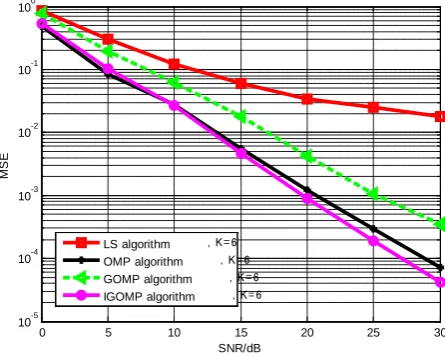
Fig.1 The MSE comparison of different algorithms

Channel reconstruction algorithms are all adopts 64 pilots. In order to make the contrast more permanent, LS

algorithm using a uniform pilot to make its performance achieve the best, and the reconstruction algorithm based on

compressive sensing adopts random pilot. The number of initialized atoms S of the GOMP algorithm and the IGOMP algorithm is 2. Simulation results are shown in

figure 1 and figure 2, they are comparison curves of mean square error and bit error rate from several different

algorithms.

0 5 10 15 20 25 30

10-4 10-3 10-2 10-1 100

SNR/dB

BER

LS algorithm ，K= 6

OMP algorithm ，K= 6 GOMP algorithm ，K= 6 IGOMP algorithm ，K= 6

Fig.2 The BER comparison of different algorithms

In the accordance with the results, with the increase of signal-to-noise(SNR) ratio, the mean square error and bit

error rate decreases in the OMP algorithm, GOMP algorithm and IGOMP algorithm. The LS algorithm is not

as good as the reconstruction algorithm based on compressive sensing. In the reconstruction algorithm based on compressive sensing, the channel reconstruction

performance of IGOMP algorithm and OMP algorithm is better than GOMP algorithm . GOMP algorithm channel

estimation performance is the worst, this is because the GOMP algorithm each time select two atoms, it may be mistaken for some extra atoms, resulting in channel

estimation performance is not good. The OMP algorithm only selects the most matching one at a time, so it is

superior to the GOMP algorithm in the reconstruction performance. When the SNR is relatively low, the channel

estimation performance of the IGOMP algorithm is slightly lower than that of the OMP algorithm. With the increase of SNR, the channel estimation performance of

IGOMP algorithm is gradually improved. In general, IGOMP algorithm performance is slightly better than

OMP algorithm, belonging to these algorithms in the best performance. This is due to the fact that IGOMP algorithm introduces a screening mechanism with an iteration stop

threshold when selecting atoms. Therefore, IGOMP algorithm performance is the best .

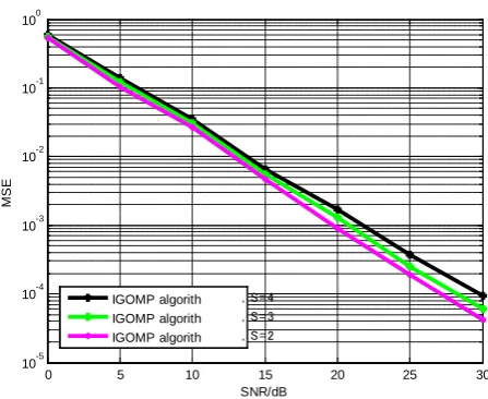
4.2 The effect of the initial step on MSE

In the processing of simulation, we need to study the effect of the original step of IGOMP algorithm to the

performance and running time of channel estimation. As is shown in figure 3, it compared the effect of IGOMP initial

step on MSE when S is 2, 3 and 4. The conclusion can be drown that the step S has an effect on the performance of channel estimation. With the increase of S, the normalized

mean squared error (MSE) is reduced gradually. This shows that when the initial step is different, the channel

estimation effect is different. As the initial step increases, the mean square error of the channel estimation increases gradually. However, when the initial step increases, the

number of atoms chosen each time increases, then the time required for channel reconstruction should also change.

The effect of the time required for channel reconstruction will be studied below when the initialization step takes different values.

0 5 10 15 20 25 30

10-5 10-4 10-3 10-2 10-1 100

SNR/dB

MS

E

IGOMP algorith ，S= 4 IGOMP algorith ，S= 3

Fig.3 The effect of IGOMP initial step on MSE

4.3 The effect of increasing sparseness on channel

estimation performance

When the value of sparseness is different, the IGOMP

algorithm is compared with the OMP algorithm. Both algorithms use 64 pilots, and the sparseness of the channels is 6 and 14, respectively. As shown in figure 4, it

can be seen that the performance of the mean square error of the two algorithms decreases when the sparseness K of

the channel increases from 6 to 14. This is because the sparseness of the channel increases and the number of pilot channels does not increase. So that no sufficient channel

condition information is obtained, resulting in an increase in the error of the channel estimation.. When the channel

sparseness is 6, the IGOMP algorithm has the same mean square error as the OMP algorithm when the SNR ratio is high. However, when the sparseness of the channel

becomes 14, the overall performance of the IGOMP algorithm is better than that of the OMP algorithm.This

means that with the increase of sparseness, IGOMP algorithm can better track the channel condition, so as to carry out channel estimation. However, the OMP

algorithm can not track the channel condition very well, resulting in the channel estimation performance is not very

good.

0 5 10 15 20 25 30

10-5 10-4 10-3 10-2 10-1 100 101

SNR/dB

MS

E

OMP algorithm ，K= 6

OMP algorithm ，K= 14

IGOMP algorithm ，K= 6

IGOMP algorithm ，K= 14

Fig.4 Comparison of MSE of two different sparseness

4.4 Comparison on running time of various reconstruction algorithms.

Here is a running time comparison in the algorithms of OMP, GOMP and IGOMP. The simulation computer

configuration is as follows.

Table2 computer configuration

Configuration Parameters

Processor

ROM

Operating system

Operating environment

Intel dual-core frequency

2.7GHz processor

2GB

Windows7

MATLAB R2012a

The table3 shows the average running time of several

reconstruction algorithms based on compressive sensing. By comparison and observation, we can see that the running time of IGOMP is shorter than that of OMP and

GOMP, in addition to that, along with the increase of the initial step, IGOMP running time decreases gradually.

Known from the analysis of theory, GOMP is to select the largest number of atoms with the residual inner product, update the index set, and then update the residual. As the

GOMP algorithm to select more atoms each time, in general, GOMP algorithm needs to be the number of

iterations will be less than OMP algorithm. therefore, compared with the OMP algorithm, GOMP algorithm has a higher computing speed. With the channel sparseness

increase, GOMP algorithm requires the number of iterations will be less.The IGOMP algorithm selects

several atoms with the largest inner product of the residuals, updates the index set, and then updates the residuals. If the iteration residual is greater than the last

iteration residual, the support set increases gradually. In this case, the number of atoms selected by the iteration is increased, which makes the algorithm run time shorter

than GOMP. In the IGOMP algorithm, when the initial step size increases, the run time is shortened due to the

increase in the number of atoms selected each time.

Table3 Running time for different algorithms

Algorithm Running Time

OMP

GOMP(S=2)

IGOMP(S=2)

IGOMP(S=3)

IGOMP(S=4)

0.0134

0.0094

0.0058

0.0050

0.0046

5.

Conclusion

In this paper, IGOMP algorithm is proposed for the

shortcomings of GOMP algorithm in OFDM channel estimation. When the number of pilot and the

signal-to-noise ratio is the same, adopting the IGOMP algorithm is not only good for channel reconstruction performance, but also for reconstruct the signal under

the condition of unpredicted sparseness, except of that, its running time is relatively short and has certain

practicality.

References

[1] DING Jing-xiao, WANG Ke-ren, CHEN Xiao-bo. Sparse Channel

Estimation Algorithm Based on OMP in OFDM Systems[J].

Communication Countermeasures, 2012, 31(1): 6-11.

[2] PENG Yu, HOU Xiao-yun, WEI Hao. Domain-Doppler Doubly

Selective Channel Estimation Using Compressed Sensing[J].

Journal of Signal Processing, 2014, 30(1): 119-126.

[3] Lang Tong, Sadler BM, Dong Min. Pilot-assisted wireless

transmissions: general model, design criteria, and signal

processing[J]. Signal Processing Magazine, IEEE, 2004, 21(6):

12-25.

[4] Lin, J-C. Least-squares channel estimation assisted by

self-interference cancellation for mobile pseudo-random-postfix

orthogonal-frequency division multiplexing applications[J].

Communications, IET, 2009, 3(12): 1907-1918.

[5] Davenport M.A, Boufounos P T, Wakin M B, et al. Signal

processing with compressive measurements[J]. IEEE Journal of

Selected Topics in Signal Processing, 2010, 4(2): 445-460.

[6] Chen Yu, Wei Yuan, Liang Yan, et al. High-Performance Sparse

Channel Estimator for OFDM System with IQ Imbalances[J].

Journal of Data Acquisition and Processing, 2014, 29(6): 986-991

[7] ZHU Xing-tao, LIU Yu-lin, XU Shun, et al. An OFDM sparse

channel estimation algorithm based on matching pursuit[J]. Journal

of Microwaves, 2008, 24 (2): 73-76.

[8] HE Xue-yun, SONG Rong-fang, ZHOU Ke-qin. Study of

compressive sensing based sparse channel estimation in OFDM

systems[J]. Journal of Nanjing University of Posts and

Telecommunications(Natural Science Edition), 2010, 30(2): 60-65．

[9] Wang J, Kwon S, Shim B. Generalized Orthogonal Matching

Pursuit[J]. IEEE Transactions on Signal Processing, 2012, 60:

6202—6216.

[10] Tong L, Sadler B M, Dong M. Pilot-assisted wireless

transmissions: general model, design criteria, and signal

processing[J]. Signal Processing Magazine IEEE, 2004, 21(6):

12-25.

YuanHang Liu, was born in Nanyang of Henan province in

1990. He is now a graduate student in Chongqing University of

Posts and Telecommunications. His research concerns mobile

communication techniques.

ZongGang Ye, was born in Xinyang of Henan province in

1989. He is now a graduate student in Chongqing University of

Posts and Telecommunications. His research concerns mobile

communication techniques.

Shuai Peng, was born in Nanchong of Sichuan province in

1991. He is now a graduate student in Chongqing University of

Posts and Telecommunications. His research concerns Mobile