The zero crossing problem

(1)

VICTORIA

~

UNIVERSITY

DEPARTMENT

OF

COMPUTER AND MATHEMATICAL

SCIENCES

The Zero Crossing Problem

A. Sofo

A. Jones (Department of Mathematics

La Trobe University)

(2'MATH{)

May 1993

TECHNICAL REPORT

VICTORIA UNIVERSITY OF TECHNOLOGY

BALLARAT ROAD (P 0 BOX 64) FOOTSCRAY

VICTORIA, AUSTRALIA 3011

TELEPHONE (03) 688-4249/4492

FACSIMILE (03) 687-7632

Campuses at

Footscray, Melton,

St Albans, Werribee

... ...

(2)

THE ZERO CROSSING PROBLEM

A. SOFO

DEPARTMENT OF COMPU1ER AND MA1HEMATICAL SCIENCES VICTORIA UNIVERSITY OF TECHNOLOGY,

MELBOURNE, AUSTRALIA

A.JONES

DEPARTMENT OF MA1HEMATICS LATROBE UNIVERSITY, MELBOURNE, AUSTRALIA

(3)

THE ZERO CROSSING PROBLEM

Abstract

We analyze a second order nonlinear differential equation that is useful in the zero crossing problem. We show that our calculated values are in agreement with the simulated values in the region of time 't, 0.1 < 't < 0.9.

Intro du ctj on

Consider a sample function of a random process as shown.

Researchers have been particularly interested in the statistics of the points where the sample function crosses the zero-axis, and in the probability density function of the intervals between these crossings.

Kac [1] in 1943 initiated some of the early investigations into this area, and more recently by Barnett [2]. Wong [3] has obtained some results based on approximate techniques.

The zero-crossing problem is a long standing one and it concerns the problem of determining the relevant statistics of the zero-crossings of random communication signals. This problem has relevance not only in communication theory, but also in the study of ocean waves, random vibrations, earthquakes, speech recognition, signal processing and frequency measurements.

Seumahu (4], through the application of the z-transformation has been able to derive a second order non-linear differential equation in the z-domain.

(4)

The Equation

Suppose that p₀is the probability that there are exactly n zero-crossings in a unit of time interval and that p is the generating function defined by

which is convergent for zE [-1, 1] and that p is twice differentiable term by term so that

then Seumahu [ 4 ], has derived the relation

" p

=

with

2 ( 2 '2) cµ P\~

-

p

co

p(l)

=

~

p₀

=

1

I

p(l)

=

~

co

p(-1)

=

~

(-1)

0

p₀

=

r

zE[-1, 1]

..•... (1)

... (2)

where c, µ,~are non-negative constants and r is a correlation coefficient such that rE [-1, 1].

(5)

Anahsis

One simple non-zero solution of (1) is obtained by inspection by noting that

(p')2 = ~2.

Note p(z) = 0 is trivial hence, using (2)

p(z)

=

~(z -1) + 1, where r

=

1 -2~

Now, a first integral of (1) can be obtained as follows:

p

=

q

2 ( 2 2)

cµ p ~ -q

Consider w = p2 and x

=

~2 • q2

'

dw -p

dx

=

--;-q

substitute for q, hence

now

so that

replace w and x

dw

dx

=

-µ\1 - w) + (1 - c)x 2

cµ x

d ( .1/c) _

- wx

-dx

(1-c)x.1/c

2 cµ

W = - X 1/c

- + l + B x 2

µ

- 1 .1/c

x

c

··· (3)

... (4)

B is a constant

... (5)

A is a new constant

(6)

Substitute into ( 4) and we have

p

=

q

q =

µp

_{... (6)}

µp

or

provided that f}2 - q2 ,. 0 which is always the case if r ,. 1 - 2fl.

Also from the initial data, we can deduce that the constant A satisfies the inequality

~f3

2

_-q

2

₎

st ;

VzE(-1,1] ....•.... (7)

More over, it follows that

(i) p(z) is a Convex function of z whenever p(z) is positive and

(ii) p(z) is a Concave function of z whenever p(z) is negative.

This leads to the following theorem.

1HEOREM

The constant of integration A, which appears in the first integral (5), of equation (1) has the

property that

and

A 2: O if r 2: r₀

(7)

5. PROOF

Consider A O!: 0, since the case A s 0 follows by reversing all the subsequent inequalities putting (5) into (1), we can write

"

p (z) =

2

µp

A 2 2

1--(f3

-q

c

1

--1

) c

the inequality at (7) now suggests that

" 2 p (z) O!: µ p

multiplying by Cosh µz, we have

integrating w.r.t. z and using p1(1) =

f3,

we have

f3

Cosh µ - µ Sinh µ O!: p' Cosh µz - µp Sinh µz

( f3

Cosh µ - µ Sinh

µ)

Sech

2

µz O!:

ci1z.

{p Sech µz} .

Integrating w.r.t. z and using the boundary condition p(l)

=

1, yields

p(z) :.

~~ ~

- [

* -

tanh

fl]

Sinh µ (1 -z)

From the other boundary condition p(-1)

=

r, we have that

r

=

p(- 1) O!: Cosh 2 µ -

1!.

Sinh 2 µ • r 0

µ

The proof is now complete.

A parametric solution of (1) from the first integral (5) can be obtained as follows:

( 2 2)

lk

p2

=

1-

f3

~q

+

~(f32-q2)

.

write

(8)

Define

··· (8)

hence

' H(q) q

p

=

2q

and

'

l = H (q) dq 2qJH(q)

dZ

since p

=

JH(q) .

Given that p1(l) =

13

integrate, with respect to the variable z.

q '

z = 1 +

I

H ( q) dq

P 2q JH(q)

q

z

=

1

+

J

!

! [

JH

(x)]

dx

x=~

z = 1 +

[ff{;5 -

/H(i)

+

Jq

[fiW

dx

q

~ x2

x=P

...

From (8), H(l3)

=

1, so that

q

z

=

1 -

~

+

[ff{;5

+

J

[fiW

dx.

13

q x2

x=P

For the special case of A • 0, the solution of (1) follows from (5)

' dp

J

2 2 2 2 q

=

p

= -

=13 -

µ

+

µ p

dz

f

dp

z

=

Jnz

2 2 2

(9)

Case (i) If

f3

= µ > 0

p(z)

=

exp( f3(z -

1)]

for xE [-1, 1]

provided that r

=

exp(-2~).

Case (ii) If

f3

> µ > 0

l/2

( f32

2)

p(z)

=

-

µ Sinh µ

(z - zo)

µ

where

provided that

z

0

=

1 -

2....

_2µ log (

f3

_{f3 -}

+ _µ

µ)

r = r

0

=

Cosh 2µ -

Ji

_µ Sinh 2µ.

[Note that the singular solution (3) corresponds to letting µ -. O]

Case (iii) If 0 <

f3

< µ

l/2

( 2 f32)

p(z)

=

µ - Cosh

µ(z - zo)

µ

where

2n

= 1 -

2 ~

log ( :

~:)

provided that

(10)

Numerical Results

For 0 < c < 1, the right hand side of (6) is continuous in a neighbourhood of p

=

1, q

=

13,

hence has a solution. Moreover, for 0

<

c

<

±•

it is differentiable and hence there is a

unique solution satisfying the given initial conditions. Thus the solution of the initial value problem

(1) is not unique. There is an infinite family of solutions, one for each choice of the constant A.

Thus we have two independent parameters c and A (regarding µ and

13

as fixed) to be detennined

from the one boundary condition p = r when

z

= -1.

For 0.1<t<0.9, the following computer method has been used to estimate the constant A (but

unfortunately does not apply for larger values of 1:).

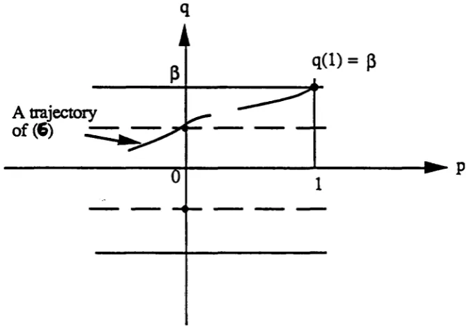
q

q(l) =

13

A trajectory

of(6)

1

Fig. 1: Singularities of the system (6)

A trajectory of the system (6) can only cross the singularities (dotted line - Fig. 1) at a point on the

q-axis. This gives the formula for A in terms of c.

l.1

(

~c

A=c

Jl}

(11)

9.

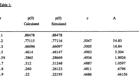
Table 1:

p(O) p(O) c A

Calculated Simulated

.1 .88478 .88478

.2 .77115 .77116 .5047 54.83

.3 .66096 .66097 .5005 16.84

.5 .4614 .46147 .4963 3.304

.59 .3865 .38669 .4936 1.8926

.7 .312 .31248 .4887 1.0597

.8 .260 .26123 .4811 .6796

.9 .22 .22195 .4686 .46156

For larger values of "C we lose the singularities, hence there is no sensible way to determine A

in terms of c. We now have two parameters but only one boundary condition to determine them.

If t = 1.2

c

= .4

~-}

p( -1) = .08063

A = .145338 p(O)

=

.11996

c

= .41

,_

}

p(-1) = .08162 gives

p(O) .12622

A = .151324

=

c

= .42

~v~}

p(-1) = .08026

A = .157272 p(O) = .132186

c

= .43

~v~}

p(-1) = .080319

A = .163124 p(O) = .137866

c

= .44

~v~}

p(-1) = .080752

A = .169025 p(O) = .137866

c

= .45

giv~}

p(-1) = .079568

(12)

Fori: = 1.2, the simulated value ofp(O) is in fact .14019.

Hence the problem in hand is 'how do we determine the parameter A in terms of c

(13)

References

[1] Kac, M., 'On the average number of real roots of a random algebraic equation'

Bull. Amer. Math. Soc. Vol. 49, p314-320, 1943.

[2] Barnett, J.T., 'Zero-crossing rates of functions of Gaussian processes.' Transactions on information theory, Vol. 37, no. 4, p1188-1194, 1991.

11.

[3] Wong, E., 'The distribution of intervals between zeros for a stationary Gaussian process.' S.I.A.M. J. Appl Math. Vol. 18, p67-73, 1970.

(4] Seumahu, E., 'Solving the zero-crossing problem through the Z Transformation.'

LaTrobe University - Technical report 1981.

[5] Gopalsamy, K., and Lalli, B., ' Necessary and sufficient conditions for zero crossing in integrodifferential equations.'

(14)