doi:10.1155/2010/102484
Research Article
Uniform Second-Order Difference
Method for a Singularly Perturbed Three-Point
Boundary Value Problem
Musa C
¸ akır
Department of Mathematics, Faculty of Sciences, Y ¨uz ¨unc ¨u Yil University, 65080 Van, Turkey Correspondence should be addressed to Musa C¸ akır,[email protected]
Received 21 June 2010; Accepted 15 October 2010 Academic Editor: Paul Eloe
Copyrightq2010 Musa C¸ akır. This is an open access article distributed under the Creative Commons Attribution License, which permits unrestricted use, distribution, and reproduction in any medium, provided the original work is properly cited.
We consider a singularly perturbed one-dimensional convection-diffusion three-point boundary value problem with zeroth-order reduced equation. The monotone operator is combined with the piecewise uniform Shishkin-type meshes. We show that the scheme is second-order convergent, in the discrete maximum norm, independently of the perturbation parameter except for a logarithmic factor. Numerical examples support the theoretical results.
1. Introduction
We consider the following singularly perturbed three-point boundary value problem:
Lu:ε2ux εaxux−bxux fx, 0< x < , 1.1
u0 A, L0u:u−γu1 B, 0< 1< , 1.2
where ε ∈ 0,1 is the perturbation parameter, and,A, B,and γ are given constants. The functionsax≥0,bx≥β >0 andfxare sufficiently smooth. For 0< ε1 the function uxhas in general boundary layers atx0 andx.
Differential equations with a small parameter 0< ε1 multiplying the highest order derivatives are called singularly perturbed differential equations. Typically, the solutions of such equations have steep gradients in narrow layer regions of the domain. Classical numerical methods are inappropriate for singularly perturbed problems. Therefore, it is important to develop suitable numerical methods to these problems, whose accuracy does not depend on the parameter value ε; that is, methods that are convergence ε-uniformly
1–5. One of the simplest ways to derive such methods consists of using a class of special piecewise uniform meshesa Shishkin mesh,see, e.g., 4–8for motivation for this type of mesh, which are constructed a priori in function of sizes of parameterε, the problem data, and the number of corresponding mesh points.
Three-point boundary value problems have been studied extensively in the literature. For a discussion of existence and uniqueness results and for applications of three-point problems, see 9–12and the references cited in them. Some approaches to approximating this type of problem have also been considered 13,14. However, the algorithms developed in the papers cited above are mainly concerned with regular casesi.e., when boundary layers are absent. Fitted difference scheme on an equidistant mesh for the numerical solution of the linear three-point reaction-diffusion problem have been studied in 15. A uniform finite difference method, which is first-order convergent, on an S-meshShishkin type meshfor a singularly perturbed semilinear one-dimensional convection-diffusion three-point boundary value problem have also been studied in 16.
Computational methods for singularly perturbed problems with two small parameters have been studied in different ways 17–21. In this paper, we propose the hybrid scheme for solving the nonlocal problem 1.1-1.2, which comprises three kinds of schemes, such as Samarskii’s scheme 22, a finite difference scheme with uniform mesh, and finite difference scheme on piecewise uniform mesh. The considered algorithm is monotone.
We will prove that the method for the numerical solution of the three-point boundary value problem 1.1-1.2 is uniformly convergent of order N−2ln2N on special piecewise
equidistant mesh, in discrete maximum norm, independently of singular perturbation parameter. InSection 2, we present some analytical results of the three-point boundary value problem1.1-1.2. InSection 3, we describe some monotone finite-difference discretization and introduce the piecewise uniform grid. In Section 4, we analyze the convergence properties of the scheme. Finally, numerical examples are presented inSection 5.
Notation 1. Henceforth,Cdenote the generic positive constants independent ofεand of the mesh parameter. Such a subscripted constant is also independent ofεand mesh parameter, but whose value is fixed.
Assumption 1. In what follows, we will assume that ε ≤ CN−1, which is nonrestrictive in practice.
2. Properties of the Exact Solution
Lemma 2.1. Ifa, b, andf∈C2 0, , the solution of 1.1-1.2satisfies the following estimates:
u∞≤C,
ukx≤C
1 1 εk
e−μ1x/εe−μ2−x/ε
, 0≤x≤, k1,2,3,4, 2.1
provided thatbx−εax≥β∗>0and|γ|<1,where
μ1
1 2
a20 4β
∗a0 ,
μ2 1
2
a2 4β∗−a .
2.2
Proof. The proof is almost identical to that of 16,23.
3. Discretization and Piecewise Uniform Mesh
Introduce an arbitrary nonuniform mesh on the segment 0,
ωN{0< x1<· · ·< xN−1< },
ωNωN∪ {x00, xN }.
3.1
Lethixi−xi−1be a mesh size at the nodexiandi hihi1/2 be an average mesh size.
Before describing our numerical method, we introduce some notation for the mesh functions. Define the following finite differences for any mesh functionvivxigiven onωNby
vx,i vi−vi−1
hi , vx,i
vi1−vi
hi1 , vx,i0
vx,ivx,i
2 ,
vx,i vi1−vi
i , i
hihi1
2 , vxx,i
vx,i−vx,i
,
w∞≡ w∞,ωN :0≤maxi≤N|wi|.
3.2
For equidistant subintervals of the mesh, we use the finite differences in the form
vx,i vi−vi−1
h , vx,i
vi1−vi
h , vxx,i
vx,i−vx,i
h . 3.3
To approximate the solution of 1.1-1.2, we employ a finite difference scheme defined on a piecewise uniform Shishkin mesh. This mesh is defined as follows.
We divide each of the intervals 0, σ1and −σ2, intoN/4 equidistant subintervals,
divisible by 4. The transition pointsσ1andσ2, which separate the fine and coarse portions of
the mesh, are obtained by taking
σ1min
4, μ
−1 1 εlnN
, σ2min
4, μ
−1 2 εlnN
, 3.4
whereμ1andμ2are given inLemma 2.1. In practice, we usually haveσi i1,2, and so
the mesh is fine on 0, σ1, −σ2, and coarse on σ1, −σ2. Hence, if we denote the step
sizes in 0, σ1, σ1, −σ2, and −σ2, byh1,h2,andh3, respectively, we have
h1 4σ1
N , h
2 2−σ2−σ1
N , h
3 4σ2
N , h
21
2
h1h3 2 N,
hk≤N−1, k1,3, N−1≤h2<2N−1,
3.5
so that
ωN
xiih1, i0,1, . . . ,N
4 ;xiσ1
i−N
4 h
2, i N
4 1, . . . , 3N
4 ;
xi−σ2
i−3N
4 h
3, i 3N
4 1, . . . , N, h
1 4σ1
N , h
2 2−σ2−σ1
N ,
h3 4σ2 N
.
3.6
On this mesh, we define the following finite difference schemes:
Lh1ui≡ε2kiuxx,iεaiux,i−biuifi−R1i , fori1,2, . . . ,N
4 −1; i 3N
4 1, . . . , N,
Lh2ui≡ε2uxx,iεaiux,i−biuifi−R2i , for i N
4 1, . . . , 3N
4 −1,
Lh3ui≡ε2uxx,i εaiux,i−biui fi−R3i , fori
N 4 ,
3N 4 ,
where
with the usual piecewise linear basis functions
ψix
It is now necessary to define an approximation for the second boundary condition of
1.2. LetxN0 be the mesh point nearest to1. Then, using interpolating quadrature formula
Substitutingx1into3.13, for the second boundary condition of1.2, we obtain
uN−γ
1−xN01 xN0−xN01
uxN0
1−xN0 xN01−xN0
uxN01
rx B. 3.15
Based on3.7and3.15, we propose the following difference scheme for approximat-ing1.1-1.2:
h1yi≡ε2kiyxx,iεaiyx,i−biyifi i1,2, . . . ,N
4 −1; i 3N
4 1, . . . , N, 3.16
h
2yi≡ε2yxx,iεaiyx,i−biyifi i N
4 1, . . . , 3N
4 −1, 3.17
h3yi≡ε2yxx,i εaiyx,i−biyifi i N
4 , 3N
4 , 3.18
y0A, 0y≡yN−γ
1−xN01 xN0−xN01
yxN0
1−xN0 xN01−xN0
yxN01
B. 3.19
4. Uniform Error Estimates
Letzy−u,x∈ωN. Then, the error in the numerical solution satisfies
hz≡Ri, i1,2, . . . , N−1,
z00, zN−γ
1−xN01 xN0−xN01
zN0
1−xN0 xN01−xN0
zN01
r,
4.1
where
RiR1i R
2
i R
3
i , 4.2
andris defined by3.14.
Lemma 4.1. Letzibe the solution to4.1. Then, the estimate
z∞,N ≤C
R∞,ωN|r|
4.3
holds.
Lemma 4.2. Under the above assumptions ofSection 1andLemma 2.1, the following estimates hold for the error functionsRiandr:
R∞,ωN ≤C
N−1lnN2,
|r| ≤CN−1lnN2.
4.4
Proof. The argument now depends on whetherσ1 σ2 /4 orσ1 μ−11 εlnN andσ2
μ−12 εlnN.In the first case
μ−11 εlnN≥ 4, μ
−1
2 εlnN≥
4, 4.5
and the mesh is uniform withh1 h2 h3 N−1for alli,1 ≤ i≤ N. Therefore, from
3.9, we have
R1i ≤C
ε2h xi1
xi−1
u4xdxεh xi1
xi−1
uxdxhxi1
xi−1
uxdx
≤C
h2
ε2
≤C
16μ−21 ln2N
2
42
N2
≤CN−1lnN2.
4.6
The same estimate is obtained forR2i andR3i in a similar manner. In the second case
μ−11 εlnN < 4, μ
−1
2 εlnN <
4, 4.7
and the mesh is piecewise uniform with the mesh spacing 4σ1/N and 4σ2/N in the
subintervals 0, σ1 and −σ2, , respectively, and 2 − σ2 − σ1/N in the subinterval
σ1, −σ2. We have the estimateR1i in 0, σ1and −σ2, and the estimateR2i in σ1, −σ2.
In the layer region 0, σ1, the estimateR1i reduces to
R1i ≤C
h1 ε
2
≤C
16μ−21 ε2ln2N
ε2N2
, 1≤i≤ N
4 −1. 4.8
Hence,
R1i ≤CN−2ln2N, 1≤i≤ N
The same estimate is obtained in the layer region −σ2, in a similar manner. We
The last two inequalities together,4.10, give the bound
Since
e−μ1xN/4−1/ε−e−μ1xN/4/εe−μ1N/4−1h1/ε
1−e−μ1h1/ε
1
N2
1−e−μ1h1/ε
< N−2,
e−μ2−xN/4/ε−e−μ2−xN/4−1/εe−μ2−xN/4/ε
1−e−μ2h1/ε
1
N2e
−μ2N/2h2/ε
1−e−μ2h1/ε
< N−2,
e−μ1xN/4/ε−e−μ1xN/41/ε 1
N2
1−e−μ1h2/ε
< N−2,
e−μ2−xN/41/ε−e−μ2−xN/4/ε 1 N2e
−μ2N/2−1h2/ε1−e−μ2h2/ε< N−2,
4.16
it then follows that
R3i ≤CN−2. 4.17
The same estimate is obtained fori3N/4 in a similar manner. This estimate is valid when only one of the values ofσ1 orσ2 is equal to/4. Next, we estimate the remainder termr.
Suppose that1∈ 2α−1ε|lnε|, −2α−1ε|lnε|, and the second derivative offon this interval
is bounded. From3.14, we obtain
|r| ≤Cfξx−xN0x−xN01
≤C|x−xN0x−xN01|
≤Ch22
≤CN−1lnN2.
4.18
Combining Lemmas 2 and 3 gives us the following convergence result.
Theorem 4.3. Letuxbe the solution of (1) andybe the solution of (29). Then, y−u
∞,N ≤CN
−2ln2
N. 4.19
5. Algorithm and Numerical Results
In this section, we present some numerical results which illustrate the present method.
aThe difference scheme3.16–3.19can be rewritten as
where
System5.1and3.19is solved by the following factorization procedure:
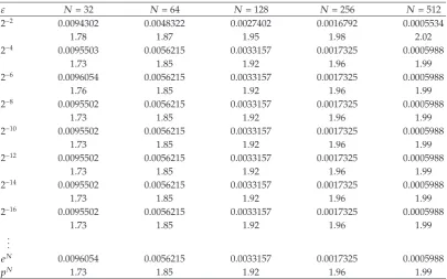
Table 1:Approximate errorseN
ε andeNand the computed orders of convergencepεNon the piecewise
uniform meshωNfor various values ofεandN.
ε N32 N64 N128 N256 N512
2−2 0.0094302 0.0048322 0.0027402 0.0016792 0.0005534
1.78 1.87 1.95 1.98 2.02
2−4 0.0095503 0.0056215 0.0033157 0.0017325 0.0005988
1.73 1.85 1.92 1.96 1.99
2−6 0.0096054 0.0056215 0.0033157 0.0017325 0.0005988
1.76 1.85 1.92 1.96 1.99
2−8 0.0095502 0.0056215 0.0033157 0.0017325 0.0005988
1.73 1.85 1.92 1.96 1.99
2−10 0.0095502 0.0056215 0.0033157 0.0017325 0.0005988
1.73 1.85 1.92 1.96 1.99
2−12 0.0095502 0.0056215 0.0033157 0.0017325 0.0005988
1.73 1.85 1.92 1.96 1.99
2−14 0.0095502 0.0056215 0.0033157 0.0017325 0.0005988
1.73 1.85 1.92 1.96 1.99
2−16 0.0095502 0.0056215 0.0033157 0.0017325 0.0005988
1.73 1.85 1.92 1.96 1.99
.. .
eN 0.0096054 0.0056215 0.0033157 0.0017325 0.0005988
pN 1.73 1.85 1.92 1.96 1.99
It is easy to verify that
Ai>0, Bi >0, Ci> AiBi, i1,2, . . . , N. 5.4
Therefore, the described factorization algorithm is stable.
bWe apply the numerical method3.16–3.19to the following problem:
ε2ux ε1cosπxux−1sinπx 2
ux fx, 0< x <1,
u0 0, u1−1 2u
1 2 1,
5.5
with
fx 2επ2cos2πx επ1cosπxsin2πx−1sinπx 2
sin2πx. 5.6
The exact solution of the problem is
ux 2 exp1−x1cosπx d/2ε "
1−expxd/ε#
−1expd/2ε−2−2 expd/2ε exp1cosπx d/4εsin
where
d
$
52 cosπx cos2πx 4 sinπx
2
. 5.8
Thisuxhas the typical boundary layers atx 0 andx 1. In the computations in this section, we take
A0, B1, γ 1
2, 1 1
2, μ12.414213562, μ21,
σ1min
1
4,2.414213562εlnN
, σ2min
1 4, εlnN
,
h2 21−σ2−σ1
N , N
∗ 0
2−4σ1Nh2
4h2
,
N0 ⎧ ⎪ ⎪ ⎪ ⎨ ⎪ ⎪ ⎪ ⎩
N0∗, if 1
2−xN0∗≤xN∗0−
1 2,
N0∗1, if 1
2−xN0∗> xN∗0−
1 2.
5.9
The error of the scheme is measured in the discrete maximum norm. For any values ofεand N, the maximum pointwise errorseN
ε and theε-uniformeNare calculated using
eNε maxi uxi−yiN, eNmaxε eNε , 5.10
whereuis the exact solution of5.5andyis the numerical solution of the finite difference scheme3.16–3.19.The convergence rates are
PεN
lneN ε /e2εN
ln 2 . 5.11
The correspondingε-uniform convergence rates are computed using the formula
PN ln
eN/e2N
ln 2 . 5.12
References
1 A. H. Nayfeh,Introduction to Perturbation Techniques, John Wiley & Sons, New York, NY, USA, 1993. 2 R. E. O’Malley Jr.,Singular Perturbation Methods for Ordinary Differential Equations, vol. 89 ofApplied
Mathematical Sciences, Springer, New York, NY, USA, 1991.
3 E. P. Doolan, J. J. H. Miller, and W. H. A. Schilders,Uniform Numerical Methods for Problems with Initial and Boundary Layers, Boole Press, Dublin, Ireland, 1980.
5 H.-G. Roos, M. Stynes, and L. Tobiska,Robust Numerical Methods for Singularly Perturbed Differential Equations, Convection-Diffusion-Reaction and Flow Problems, vol. 24 ofSpringer Series in Computational Mathematics, Springer, Berlin, Germany, 2nd edition, 2008.
6 T. Linß and M. Stynes, “A hybrid difference scheme on a Shishkin mesh for linear convection-diffusion problems,”Applied Numerical Mathematics, vol. 31, no. 3, pp. 255–270, 1999.
7 I. A. Savin, “On the rate of convergence, uniform with respect to a small parameter, of a difference scheme for an ordinary differential equation,”Computational Mathematics and Mathematical Physics, vol. 35, no. 11, pp. 1417–1422, 1995.
8 G. F. Sun and M. Stynes, “A uniformly convergent method for a singularly perturbed semilinear reaction-diffusion problem with multiple solutions,”Mathematics of Computation, vol. 65, no. 215, pp. 1085–1109, 1996.
9 R. Cziegis, “The numerical of singularly perturbed nonlocal problem,”Lietuvas Matematica Rink, vol. 28, pp. 144–152, 1988Russian.
10 R. ˇCiegis, “On the difference schemes for problems with nonlocal boundary conditions,”Informatica, vol. 2, no. 2, pp. 155–170, 1991.
11 A. M. Nakhushev, “Nonlocal boundary value problems with shift and their connection with loaded equations,”Differential Equations, vol. 21, no. 1, pp. 92–101, 1985Russian.
12 M. P. Sapagovas and R. Yu. Chegis, “Numerical solution of some nonlocal problems,” Litovski˘ı Matematicheski˘ıSbornik, vol. 27, no. 2, pp. 348–356, 1987Russian.
13 B. Liu, “Positive solutions of second-order three-point boundary value problems with change of sign,” Computers & Mathematics with Applications, vol. 47, no. 8-9, pp. 1351–1361, 2004.
14 R. Ma, “Positive solutions for nonhomogeneousm-point boundary value problems,”Computers & Mathematics with Applications, vol. 47, no. 4-5, pp. 689–698, 2004.
15 G. M. Amiraliyev and M. C¸ akir, “Numerical solution of the singularly perturbed problem with nonlocal boundary condition,”Applied Mathematics and Mechanics, vol. 23, no. 7, pp. 755–764, 2002. 16 M. Cakir and G. M. Amiraliyev, “Numerical solution of a singularly perturbed three-point boundary
value problem,”International Journal of Computer Mathematics, vol. 84, no. 10, pp. 1465–1481, 2007. 17 J. L. Gracia, E. O’Riordan, and M. L. Pickett, “A parameter robust second order numerical method
for a singularly perturbed two-parameter problem,”Applied Numerical Mathematics, vol. 56, no. 7, pp. 962–980, 2006.
18 T. Linß and H.-G. Roos, “Analysis of a finite-difference scheme for a singularly perturbed problem with two small parameters,”Journal of Mathematical Analysis and Applications, vol. 289, no. 2, pp. 355– 366, 2004.
19 T. Linß, “Layer-adapted meshes for convection-diffusion problems,”Computer Methods in Applied Mechanics and Engineering, vol. 192, no. 9-10, pp. 1061–1105, 2003.
20 C. Clavero, J. L. Gracia, and F. Lisbona, “High order methods on Shishkin meshes for singular perturbation problems of convection-diffusion type,”Numerical Algorithms, vol. 22, no. 1, pp. 73–97, 1999.
21 R. E. O’Malley Jr., “Two-parameter singular perturbation problems for second-order equations,” Journal of Mathematics and Mechanics, vol. 16, pp. 1143–1164, 1967.
22 A. A. Samarskii,Theory of Difference Schemes, M. Nauka, Moscow, Russia, 1971.