Burst Error Characterization for Wireless Ad-Hoc Network and Impact of Packet Interleaving

Burst Error Characterization for Wireless Ad-Hoc

Network and Impact of Packet Interleaving

Devaraju. R#, Puttamadappa. C*

#

Department of Electronics and Communications,

Sapthagiri College of Engineering, Visvesvaraya Technological University Bangalore, Karnataka, India

*

Sapthagiri College of Engineering, Visvesvaraya Technological University Bangalore, Karnataka, India

Abstract— Multimedia data transmission over wireless networks is challenging due lower bandwidth, delay composition, air interface and occurrence of burst errors. Packet loss caused by burst errors seriously limits the maximum achievable throughput of wireless networks. Burst errors are critical for Quality of Service (QoS) in terms of error detection, correction and retransmission of erroneous packets. Codecs for most of the multimedia traffic like voice, video transmissions are usually designed to conceal single error but not burst of packet error. To tailor efficient transmission schemes, it is essential to design a wireless error model and develop techniques that can provide insight into the behaviour of wireless transmissions.

Keywords— Burst Error, Error Model, Forward Error Correction Codes, Gilbert Model, Markov Chains, Packet Interleaving, Wireless ad-hoc Network.

I. INTRODUCTION

Error modeling in communication channels is a popular methodology used for analyzing the channel characteristics, investigating the impact of errors, testing and evaluates the methods to improve the channel performance. Communication channels can be modeled mathematically for channels with memory and without memory. Discrete Memory less channels are the simplest type of channel for which the output of the channel at any given time depends only on the corresponding input. A channel is said to have memory, if each bit in the output sequence depends statistically on the corresponding input bit as well as on the past inputs, past outputs and future inputs. In digital wireless channels burst errors are common which might occur because of the non-stationary noise effect in the transmission channel or due to stroke of lightning. Burst errors are not independent; they tend to be spatially concentrated. If one of the symbols has an error, it is likely that the adjacent symbols could also be corrupted. Describing the statistical property of the underlying burst error sequence is termed as Burst error model.

Error models can be classified either as descriptive or generative models. A descriptive model analyzes the statistical behavior of a channel for error sequence with reference to the historical events, which can be obtained from a real channel or a simulation process. Generative model specifies an algorithm or a methodology for generating the error patterns similar to the statistical error

sequences. The algorithm is based on the mathematical calculations that can accurately predict the future outcomes [1]. The detailed characterization of the digital wireless channel is very difficult. Gilberts two state model has been successful in characterizing the burst error in digital wireless channels [2]. Gilbert model is based on finite-state binary symmetric channel with memory determined by Markov chains. The two state of the channel corresponds to the channel quality which is either “good” or “bad” are represented by 0 and 1 respectively [3]. Due to the underlying Markov nature of the state process, the occurrence of symbol for the channel with memory depends on the transition between the two states. The transition probability defines the probability of transition from one state to another state in a single step and termed as P(0)and P(1)respectively [4].

To counteract the burst error losses and improve the QoS of the communication channel, the concept of interleaving technique comes very handy. Interleaving is the technique of minimizing the burst errors by transforming them into independent errors. Uniformly randomizing the burst error to independent error helps in designing a simple Forward Error Correction codes (FEC). By re-ordering the symbols before transmitting them over a channel, the symbols are separated apart with reference to interleaving depth, resulting the same code word is not hit by the same burst. The receiver performs the inverse operation called deinterleaving. If the interleaving depth is large enough, error can be treated on the de-interleaver output as independent [5]. Comparing the symbol error rates for different burst error with interleaving against the traditional communication protocol highlights the advantages.

II. DEFINITION OF BURST ERROR AND WAITING TIME

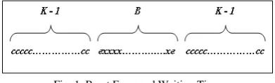
Consider a sequence of symbol output by the Viterbi decoder of the form where the codeword ‘c’ represents correctly decoded symbol, codeword ‘e’ represents an error symbol and ‘x’ may be either correct or incorrect symbol.

Fig. 1 Burst Error and Waiting Time

Suppose that there is no string of K-1 consecutive c’s in the sequence ‘xx----x’, then the string ‘exx----xe’ is called a burst error of length B. A string of c’s between the two burst is referred as a waiting time [6].

III.GILBERT MODEL

Gilbert model is a first order markov chain model, which is mainly used to study the packet loss process in a communication network. We have considered the two state binary symmetric channel models with memory for our current study. Two state good ( )G and bad ( )B are assumed in this model. In the good state error occur with very low probability p_ggwhile in bad state errors occur

with high probabilityp_bb. The channel has the opportunity to change states. The transition from GBand

BGhave probabilities 1p_ggand 1p_bbrespectively [7].

A. Two-State Gilbert Model

Digital communication systems transmit information in the form of 0and1. Each symbol transmitted should pass through several stages and routes to reach the destination node. There is probability( )P that the symbol transmitted will remain unchanged when received. We can say that the communication process is in state0when the transmitted symbol is unchanged and state1when the symbol has changed from its original value.

Two states Gand Bare said to be accessible to each other if n 0

gb

P  for valuen0

B. Definitions

G: good state with a null error probabilitypgg,

B: bad state with an error probability equal topbb,

1pgg: Probability to change from good to bad state,

1pbb: Probability to change from bad to good state.

Fig. 2 Two State Gilbert Model

Any state can communicates with itself since, by definition,





0

0 | 0 1

gg

P P X G X G 

 

₁

To simulate bursty error behaviourpggand pbbmust be

large. The transition matrix defines the general solution for linear dynamical systems. Two state gilberts model has the following state transition matrix form:

1 1

gg gg

bb bb

p p

P

p p



 

  _ 

 

 

2

Equation 2 is also called the one-step transition probability matrix. In the model, the occurrence of a symbol transmitted with or without error is modeled respectively by 1 and 0 .

Consider the example of a two-state model in which 0.7

gg

p  andpbb 0.4, then the one-step transition

probability matrix is given by

0.7 0.3 0.4 0.6

P  _

 

 

3

The one-step probability values for1pgg 0.3

and1pbb0.6. Now if we want to calculate the probability that next four symbols transmitted remain the state 0 provided the current symbol is in state 0, then

2 0.7 0.3 0.7 0.3

.

0.4 0.6 0.4 0.6

P    _{ } _

   

 

4

2 0.61 0.39

0.52 0.48

P   _

 

 

5

Similarly P4can be calculated as

 

2

4 2 0.61 0.39 0.61 0.39

.

0.52 0.48 0.52 0.48

P  P    _{ } _

   

 

6

4 0.5749 0.4215

0.5668 0.4332

P   _

 

 

7

Hence the desired probability for 4

gg

P is 0.5749.

Next observable state deals with the capability of determining the state transition from input to output while not knowing the initial state. The observational transition probability matrix for two state gilberts model is given by:

( )(1 ) (1 )(1 ) (0)

(1 )(1 ) ( )(1 )

gg gg

bb bb

p G p G

P

p B p B

  

 

  _{  } 

( )( ) (1 )( ) (1)

(1 )( ) ( )(1 )

gg gg

bb bb

p G p G

P

p B p B



 

  _{ } 

 

 

9

The stationary state probability is the probability of being in various states as time gets large. Stationary state probability is considered in many applications since one is interested in long run behavior of the system. Now under the conditions 0 1 p_ggand1p_bb1, the stationary state

probabilities ₀and ₁ of being in state Gand

Brespectively can be defined as:

0

(1 )

(1 ) (1 )

bb

gg bb

p

p p

  

  

 

10

1

(1 )

(1 ) (1 )

gg

gg bb p

p p

  

  

 

11

Therefore steady state probability can be defined as



0, 1



   

 

12

The entries of are called steady state probabilities. The average symbol error rate produced by the Gilberts channel is defined as:

0 0 1 1

pP P

 

13

Using equation 10 and 11, Equation 13 can be further simplified and defined as

0(1 ) 1(1 )

(1 ) (1 )

gg bb

gg bb

P p P p

p

p p

  



  

 

14

Using Equation 14, the average symbol error rate can be derived as

(1 )

(1 ) (1 )

bb gg bb p p p p  

  

 

15

Next, the variance of the error symbol Xis the average value of the square distance from the mean value. It represents how the random variable is distributed near the mean value. Small variance indicates that the random variable is distributed near the mean value while big variance indicates that the random variable is distributed far from the mean value. Standard equation of variance is given by

2 2

( )

E X p

  

 

16

In the current context variance is defined as

2

(1 )

p p

  

 

17

The correlation will indicate a predictive relationship that can be exploited in practice. The correlation coefficient of two consecutive error symbols X1and X2is defined as:



1 2



2

( )( )

E X p X p





 



 

18

Equation 18 can be further simplified and rewritten as

1

bb gg

p p

  

 

19

Solving equations 15 and 19, we get the bad state probability as

(1 )

bb

p  p  p

 

20

And the good state probability is derived as

(1 )

gg

p  p p

 

21

The transition probability matrix then becomes:

1 (1 ) (1 )

(1 )(1 ) 1 (1 )(1 )

p p P p p            _{    } 

 

 

22

The nthstep transition matrix may be obtained by multiplying the matrix Pby itself ntimes.

Referring to equation 7, it is evident that asn 

,

the desired probability converge towards a particular value. Also there seems to be a limiting probability that the communication process will be in any particular state after a long number of transitions and this value is independent of the initial state.

IV.INTERLEAVING

In our current study we have considered Block Interleaver, which is a variant of periodic interleaver. In a block interleaver the flow of symbols is divided in sequence of K symbols. Each of the sequence is then placed into a matrix form of sizen m , where n represents the number of rows and is called interleaving depth and m

represents the columns and referred as block size. A sample sequence of symbols in a 4 4 matrix is represented in figure 3.

Symbols are read into the matrix by rows and read out by columns. For continuous interleaving two matrices are required. Symbols are written into one matrix whilst they are read out of the other. This clearly leads to the considerable delay in the interleaver, with output of symbol from the buffer matrix being delayed until all symbols have been read in.

Fig. 3 n m Block Interleaver

The rearrangement of symbols by the interleaver is such that if mor fewer symbols are lost from a block, each original group of nsymbols after deinterleaving will contain at most one loss. Sample codeword sequence along with random burst error is demonstrated in the figure 4.

Fig. 4 Block Interleaver and De-interleaver

It can be noticed that the grey colored symbols are the random burst errors, which are expected to occur in the communication channel. When the de-interleaving technique is applied on the above sequence the burst errors are distributed in such a way that it contains at most one packet error.

The burst error Aof length Bwill be converted in

smaller burst of lengthB

n. In ideal case, when nBwe are

able to convert the burst in an equivalent number of isolated losses spaced of mor m1symbols. Therefore, increasing nand m, the capacity of converting burst into isolated losses increases.

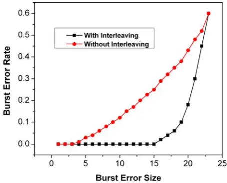
Figure 5 compares the symbol error rates for different burst error size with interleaving against the traditional communication protocol.

Fig. 5 Trial results with and without Interleaving

Error rates when compared for communication channel with and without interleaving clearly indicates that the QoS in terms of error detection, correction and retransmission of erroneous packets can be optimized using simple and efficient FEC algorithms.

The interleaving technique can be applied at different levels, which range from the bit/byte to an entire frame of a video stream. We decided to work at packet level as the losses on the internet majorly happen at packet level and considering the flexibility of internet protocol, it is not fixed to any particular technology.

Generally, the interleaver follows a relationship from its input xk to it output xk of

( )

k k

x x

 

23

Where ( )k is the function that describes the mapping of interleaver output time indices to interleaver input time indices.

Because of the periodicity,

( )k L (k L)

   

 

24

The interleaving depth ‘J’ can be mathematically defined using the function  as

1 1

0... 1

( ) ( 1)

min

k L

J  k  k

 

  

 

25

V. EFFECT OF SYMBOL INTERLEAVING

If the code is interleaved to degree' 'L , then Lcode words are grouped together and the symbols are transmitted in an order such that the _Jth

transmitted symbol belongs to code wordi.

0  i L 1

 

26

Where Ji(mod )L

Without interleaving(L1), the transitional probabilities associated with the transmission of two consecutive symbols in a particular codeword are given by equation 2.

When the codeword is interleaved to degreeL1, two consecutive symbols of a codeword are spaced apart by

Lsymbols times.

Then the corresponding transitional probability for these two symbols is given by the matrix L

P . For a model interleaved to degreeL, the transition probability matrix equals the transition probability matrix for the un-interleaved model given by Equation 22 with replaced

byL

.

(1 )(1 ) (1 )

(1 )(1 ) 1 (1 )(1 )

L L

L

L L

p p

P

p p

 

 

    

  

    

 

 

27

The results say that interleaving to degree' 'L has the effect of raising the correlation co-efficient of the channel to the Lthpower [8]. The crossover probability for this interleaving is given by equation 20 and equation 21 as follows:

(1 )

L L bb

p  p  p

 

28

(1 )

L L

gg

p  p  p

 

29

It is evident that asL ;pbbL p and 1 L gg

p  . The bit error remains unaltered. The burst errors are distributed in such a way that it contains at most one packet error. This will result in designing a simple error detection and correction algorithms.

VI.RESULTS AND DISCUSSIONS

We have performed series of experiment trials with the parameter values listed in the table 1. The parameter values used for the experiments are derived from the equations discussed in the early part of this paper.

Consider the one-step transition probability matrix for the two state Gilberts model from equation 3, wherep_gg 0.7,p_bb0.4,1p_gg 0.3 and1p_bb0.6.

Using the above values form one-step transition probability matrix in equations 10 and 11, we get the stationary state probabilities0and1as

0 (0.6)

0.666 (0.9)

  

_{ }

30

1 (0.3)

0.333 (0.9)

  

 

31

Now the correlationfrom equation 19 will be

1 0.4 0.7 1 0.1

bb gg

p p

      

 

32

Now all the resultant values from equations 30, 31, 32 along with the static trial values are tabulated in the table 1.

TABLEI

PARAMETERS USED FOR THE EXPEREMENT TRIALS

Parameter Values

InterleavingBlockSize [12,16]

InterleavingDepth [3, 4]

( )

b Loss

 [0.333]

(Correlation)

 [0.1]

Trials [12]

Protocols [udp tcp rtp, , ]

PayloadSize [512]

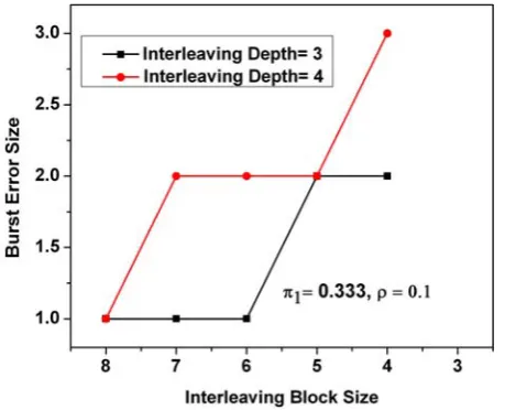
Figure 6 demonstrates the burst error randomization for different values of interleaving depth having the same loss probability and correlation factor. Increasing the correlation factor results in higher error bursts which intern results in more effective interleaving process. Also it can be noticed that increasing the interleaving depth, the desired probability converge towards a particular value. Any further increase in interleaving depth beyond this point will be similar to the channel with no memory and provides no additional benefits.

VII. SUMMARY

In this paper, we studied the evaluation of burst errors in symbol transmission by modeling the communication channel. Gilbert’s model which is the first order markov chain model is used to study the packet loss process. The accuracy of using Gilbert’s error model was compared and justified against the analytical results. Concept of symbol interleaving was introduced to uniformly randomizing the burst errors to independent error. Performance of different symbol codes was verified to see the effect of interleaving. Experiment confirms that increasing the correlation factor results in higher burstiness. Simultaneously increasing the interleaving depth, the desired probability converges towards a particular value and any further increase provides no additional benefits. We have also demonstrated that the error rates when compared for communication channel with and without interleaving clearly indicates that the QoS in terms of error detection, correction and retransmission of erroneous packets can be optimized using simple and efficient FEC algorithms.

REFERENCES

[1] Chengxaing Wang, Dayong Xu, “A Study of Burst Error Statistics and Error Modeling for MB-OFDM UWB Systems,” Ultra Wideband Systems, Technologies and Applications, April 2006, pp 244 - 248.

[2] S. Srinivas, K.S. Shanmugam, “Markov Models for Burst Errors in Radio Communications Channels,” Wireless Personal Communications, The Springer International Series in Engineering and Computer Science Volume 262, 1994, pp 175 - 184.

[3] Hong Shen Wang, Nader Moayeri, “Finite-State Markov Channel – A Useful Model for Radio Communication Channels,” IEEE Transactions on Vehicular Technology, Vol. 44, No. 1, February 1995, pp 163 - 171.

[4] Mohammad Rezaeian, “Computation of Capacity for Gilbert-Elliott Channels, Using a Statistical Method,” Communications Theory Workshop, February 2005, pp 56 – 61.

[5] Ling-Jyh Chen, Tony Sun, M. Y. Sanadidi, Mario Gerla, “Improving Wireless Link Throughput via Interleaved FEC,” Computers and Communications, July 2004, pp 539 – 544.

[6] L. J. Deutsch, R. L. Miller, “Burst Statistics of Viterbi Decoding,” TDA Progress Report, June 1981, pp 41 – 64.

[7] James R. Yee, Edward J. Weldon Jr, “Evaluation of the Performance of Error-Correcting Codes on a Gilbert Channel,” IEEE Transactions on Communications, Vol. 43, No. 8, AUGUST 1995, pp 2316 – 2323.