Identifying Cross-Document Relations between Sentences
Yasunari Miyabe†§ Hiroya Takamura‡ Manabu Okumura‡
†Interdisciplinary Graduate School of Science and Engineering,
Tokyo Institute of Technology, Japan
‡Precision and Intelligence Laboratory,
Tokyo Institute of Technology, Japan
[email protected], {takamura,oku}@pi.titech.ac.jp
Abstract
A pair of sentences in different newspaper articles on an event can have one of sev-eral relations. Of these, we have focused on two, i.e., equivalence and transition. Equiv-alence is the relation between two sentences that have the same information on an event. Transition is the relation between two sen-tences that have the same information except for values of numeric attributes. We pro-pose methods of identifying these relations. We first split a dataset consisting of pairs of sentences into clusters according to their similarities, and then construct a classifier for each cluster to identify equivalence re-lations. We also adopt a “coarse-to-fine” ap-proach. We further propose using the identi-fied equivalence relations to address the task of identifying transition relations.
1 Introduction
A document generally consists of semantic units called sentences and various relations hold between them. The analysis of the structure of a document by identifying the relations between sentences is called
discourse analysis.
The discourse structure of one document has been the target of the traditional discourse anal-ysis (Marcu, 2000; Marcu and Echihabi, 2002; Yokoyama et al., 2003), based on rhetorical struc-ture theory (RST) (Mann and Thompson, 1987).
§Yasunari Miyabe currently works at Toshiba Solutions Cor-poration.
Inspired by RST, Radev (2000) proposed the cross-document structure theory (CST) for multi-document analysis, such as multi-multi-document summa-rization, and topic detection and tracking. CST takes the structure of a set of related documents into ac-count. Radev defined relations that hold between sentences across the documents on an event (e.g., an earthquake or a traffic accident).
Radev presented a taxonomy of cross-document relations, consisting of 24 types. In Japanese, Etoh et al. (2005) redefined 14 CST types based on Radev’s taxonomy. For example, a pair of sentences with an “equivalence relation” (EQ) has the same information on an event. EQ can be considered to correspond to the identity and equivalence relations in Radev’s taxonomy. A sentence pair with a “tran-sition relation” (TR) contains the same numeric at-tributes with different values. TR roughly
corre-sponds to the follow-up and fulfilment relations in Radev’s taxonomy. We will provide examples of CST relations:
1. ABC telephone company announced on the 9th that the number of users of its mobile-phone service had reached one million. Users can ac-cess the Internet, reserve train tickets, as well as make phone calls through this service.
2. ABC said on the 18th that the number of users of its mobile-phone service had reached 1,500,000. This service includes Internet ac-cess, and enables train-ticket reservations and telephone calls.
has changed from one million to 1.5 millions, while other things remain unchanged. The pair of the sec-ond sentence in 1 and the secsec-ond sentence in 2 is in EQ, because these two sentences have the same information.
Identification of CST relations has attracted more attention since the study of multi-document dis-course emerged. Identified CST types are helpful in various applications such as multi-document sum-marization and information extraction. For example,
EQ is useful for detecting and eliminating redundant
information in multi-document summarization. TR can be used to visualize time-series trends.
We focus on the two relations EQ and TR in the Japanese CST taxonomy, and present methods for their identification. For the identification of EQ pairs, we first split a dataset consisting of sentence pairs into clusters according to their similarities, and then construct a classifier for each cluster. In addi-tion, we adopt a coarse-to-fine approach, in which a more general (coarse) class is first identified before the target fine class (EQ). For the identification of TR pairs, we use variable noun phrases (VNPs), which are defined as noun phrases representing a variable with a number as its value (e.g., stock prices, and population).
2 Related Work
Hatzivassiloglou et al. (1999; 2001) proposed a method based on supervised machine learning to identify whether two paragraphs contain similar in-formation. However, we found it was difficult to accurately identify EQ pairs between two sentences simply by using similarities as features. Zhang et al. (2003) presented a method of classifying CST relations between sentence pairs. However, their method used the same features for every type of CST, resulting in low recall and precision. We thus select better features for each CST type, and for each cluster of EQ.
The EQ identification task is apparently related to Textual Entailment task (Dagan et al., 2005). Entail-ment is asymmetrical while EQ is symmetrical, in the sense that if a sentence entails and is entailed by another sentence, then this sentence pair is in EQ. However in the EQ identification, we usually need to find EQ pairs from an extremely biased dataset of
sentence pairs, most of which have no relation at all.
3 Identification of EQ pairs
This section explains a method of identifying EQ pairs. We regarded the identification of a CST re-lation as a standard binary classification task. Given a pair of sentences that are from two different but related documents, we determine whether the pair is in EQ or not. We use Support Vector Machines (SVMs) (Vapnik, 1998) as a supervised classifier. Please note that one instance consists of a pair of two sentences. Therefore, a similarity value between two sentences is only given to one instance, not two.
3.1 Clusterwise Classification
Although some pairs in EQ have quite high similar-ity values, others do not. Simultaneously using both of these two types of pairs for training will adversely affect the accuracy of classification. Therefore, we propose splitting the dataset first according to sim-ilarities of pairs, and then constructing a classifier for each cluster (sub-dataset). We call this method
clusterwise classification.
We use the following similarity in the cosine mea-sure between two sentences (s1,s2):
cos(s1, s2) =u1·u2/|u1||u2|, (1)
where u1 and u2 denote the frequency vectors of
content words (nouns, verbs, adjectives) for respec-tives1ands2. The distribution of the sentence pairs
according to the cosine measure is summarized in Table 1. From the table, we can see a large dif-ference in distributions of EQ and no-relation pairs. This difference suggests that the clusterwise classi-fication approach is reasonable.
We split the dataset into three clusters:
high-similarity cluster, intermediate-high-similarity cluster,
and low-similarity cluster. Intuitively, we ex-pected that a pair in the high-similarity cluster would have many common bigrams, that a pair in the intermediate-similarity cluster would have many common unigrams but few common bigrams, and that a pair in the low-similarity cluster would have few common unigrams or bigrams.
3.2 Two-Stage Identification Method
Table 1: The distribution of sentence pairs according to the cosine measure (NO indicates pairs with no relation. The pairs with other relations are not on the table due to the space limitation)
cos (0.0,0.1] (0.1,0.2] (0.2,0.3] (0.3,0.4] (0.4,0.5] (0.5,0.6] (0.6,0.7] (0.7,0.8] (0.8,0.9] (0.9,1.0]
EQ 12 13 21 25 37 61 73 61 69 426
summary 5 5 25 19 22 13 16 6 6 0
refinement 3 4 15 11 12 15 6 6 3 2
NO 194938 162221 68283 28152 11306 4214 1379 460 178 455
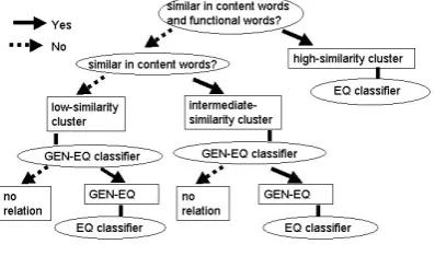
Figure 1: Method of identifying EQ pairs
smaller than the total number of sentence pairs as shown in Table 1. These two clusters also contain many pairs that belong to a “summary” and a “re-finement” relation, which are very much akin to EQ. This may cause difficulties in identifying EQ pairs.
We gave a generic name, GEN(general)-EQ, to the union of EQ, “summary”, and “refinement” re-lations. For pairs in the intermediate- or low-similarity clusters, we propose a two-stage method using GEN-EQ on the basis of the above observa-tions, which first identifies GEN-EQ pairs between sentences, and then identifies EQ pairs from
GEN-EQ pairs.
This two-stage method can be regarded as a coarse-to-fine approach (Vanderburg and Rosenfeld, 1977; Rosenfeld and Vanderbrug, 1977), which first identifies a coarse class and then finds the target fine class. We used the coarse-to-fine approach on top of the clusterwise classification method as in Fig. 1.
There are by far less EQ pairs than pairs without relation. This coarse-to-fine approach will reduce this bias, since GEN-EQ pairs outnumber EQ pairs.
3.3 Features for identifying EQ pairs
Instances (i.e., pairs of sentences) are represented as binary vectors. Numeric features ranging from 0.0
to 1.0 are discretized and represented by 10 binary features (e.g., a feature value of 0.65 is transformed into the vector 0000001000). Let us first explain ba-sic features used in all clusters. We will then explain other features that are specific to a cluster.
3.3.1 Basic features
1. Cosine similarity measures: We use unigram, bi-gram, tribi-gram, bunsetsu-chunk1similarities at all the sentence levels, and unigram similarities at the para-graph and the document levels. These similarities are calculated by replacingu1andu2in Eq. (1) with
the frequency vectors of each sentence level.
2. Normalized lengths of sentences: Given an in-stance of sentence pairs1ands2, we can define
fea-turesnormL(s1)andnormL(s2), which represent
(normalized) lengths of sentences, as:
normL(s) =len(s)/EventM ax(s), (2)
where len(s) is the number of characters in s. EventM ax(s) ismaxs0∈event(s)len(s0), where
event(s) is the set of sentences in the event that doc(s) describes. doc(s) is the document contain-ings.
3. Difference in publication dates: This feature de-pends on the interval between the publication dates ofdoc(s1)anddoc(s2)and is defined as:
DateDif f(s1, s2) = 1−|
Date(s1)−Date(s2)|
EventSpan(s1, s2)
, (3)
where Date(s) is the publication date of an arti-cle containings, andEventSpan(s1, s2)is the time
span of the event, i.e., the difference between the publication dates for the first and the last articles that are on the same event. For example, ifdoc(s1) is
published on 1/15/99 and doc(s2) on 1/17/99, and
if the time span of the event ranges from 1/1/99 to 1/21/99, then the feature value is 1-2/20 = 0.9.
1
4. Positions of sentences in documents (Edmund-son, 1969): This feature is defined as
P osit(s) =lenBef(s)/len(doc(s)), (4)
wherelenBef(s) is the number of characters be-foresin the document, andlen(doc(s))is the total number of characters indoc(s).
5. Semantic similarities: This feature is measured by Eq. (1) withu1 andu2 being the frequency vectors
of semantic classes of nouns, verbs, and adjectives. We used the semantic classes in a Japanese thesaurus called ‘Goi-taikei’ (Ikehara et al., 1997).
6. Conjunction (Yokoyama et al., 2003): Each of 55 conjunctions corresponds to one feature. If a con-junction appears at the beginning of the sentence, the feature value is 1, otherwise 0.
7. Expressions at the end of sentences: Yokoyama et al. (2003) created rules that map sentence endings to their functions. Each function corresponds to a feature. If a function appears in the sentence, the value of the feature for the function is 1, otherwise 0. Functions of sentence endings are past, present, as-sertion, existence, conjecture, interrogation, judge-ment, possibility, reason, request, description, duty, opinion, continuation, causation, hearsay, and mode.
8. Named entity: This feature represents sim-ilarities measured through named entities in the sentences. Its value is measured by Eq. (1) with u1 and u2 being the frequency vectors of the
named entities. We used the named-entity chun-ker bar2. The types of named entities are ARTI-FACT DATE ORGANIZATION MONEY LO-CATIONTIMEPERCENTand PERSON.
9. Types of named entities with particle: This fea-ture represents the occurrence of types of named en-tities accompanied by a case marker (particle). We used 11 different case markers.
3.3.2 Additional features to identify fine class
We will next explain additional features used in identifying EQ pairs from GEN-EQ pairs.
1. Numbers of words (morphemes) and phrases: These features represent the closeness of the num-bers of words and bunsetsu-chunks in the two sen-tences. This feature is defined as:
2
http://chasen.naist.jp/˜masayu-a/p/bar/
N umW(s1, s2) = 1− |
f rqW(s1)−f rqW(s2)|
max(f rqW(s1), f rqW(s2))
, (5)
wheref rqW(s)indicates the number of words in s. Similarly, N umP(s1, s2)is obtained by
replac-ing f rqW in Eq. (5) with f rqP, where f rqP(s) indicates the number of phrases ins.
2. Head verb: There are three features of this kind. The first indicates whether the two sentences have the same head verb or not. The second indicates whether the two sentences have a semantically sim-ilar head verb or not. If the two verbs have the same semantic class in a thesaurus, they are re-garded as being semantically similar. The last in-dicates whether both sentences have a verb or not. The head verbs are extracted using rules proposed by Hatayama (2001).
3. Salient words: This feature indicates whether the salient words of the two sentences are the same or not. We approximate the salient word with the ga-or the wa-case wga-ord that appears first.
4. Numeric expressions and units (Nanba et al., 2005): The first feature indicates whether the two sentences share a numeric expression or not. The second feature is similarly defined for numeric units.
4 Experiments on identifying EQ pairs
We used the Text Summarization Challenge (TSC) 2 and 3 corpora (Okumura et al., 2003) and the Work-shop on Multimodal Summarization for Trend Infor-mation (Must) corpus (Kato et al., 2005). These two corpora contained 115 sets of related news articles (10 documents per set on average) on various events. A document contained 9.9 sentences on average. Etoh et al. (2005) annotated these two corpora with CST types. There were 471,586 pairs of sentences and 798 pairs of these had EQ. We conducted the experiments with 10-fold cross-validation (i.e., ap-proximately 425,000 pairs on average, out of which approximately 700 pairs are in EQ, are in the train-ing dataset for each fold). The average, maximum, and minimum lengths of the sentences in the whole datset are shown in Table 2. We used precision, recall, and F-measure as evaluation measures. We used a Japanese morphological analyzer ChaSen3to
3
Table 2: Average, max, min lengths of the sentences in the dataset
average max min
# of words 33.27 458 1
# of characters 111.22 1107 2
extract parts-of-speech. and a dependency analyzer CaboCha4to extract bunsetsu-chunks.
4.1 Estimation of threshold
We split the set of sentence pairs into clusters ac-cording to their similarities in identifying EQ pairs as explained. We used 10-fold cross validation again
within the training data (i.e., the approximately
425,000 pairs above are split into a temporary train-ing dataset and a temporary test dataset 10 times) to estimate the threshold to split the set, to select the best feature set, and to determine the degree of the polynomial kernel function and the value for soft-margin parameterCin SVMs. No training instances are used in the estimation of these parameters.
4.1.1 Threshold between high- and intermediate-similarity clusters
We will first explain how to estimate the threshold between high- and intermediate-similarity clusters.
We expected that a pair in high-similarity cluster would have many common bigrams, and that a pair in intermediate-similarity cluster would have many common unigrams but few common bigrams. We therefore assumed that bigram similarity would be ineffective in intermediate-similarity cluster.
We determined the threshold in the following way for each fold of cross-validation. We decreased the threshold by 0.01 from 1.0. We carried out 10-fold cross-validation within the training data, excluding one of the 14 features (6 cosine similarities and other basic features) for each value of the threshold. If the exclusion of a feature type deteriorates both av-erage precision and recall obtained by the cross-validation within the training data, we call it
ineffec-tive. We set the threshold to the minimum value for
which bigram similarity is not ineffective. We obtain a threshold value for each fold of cross-validation. The average value of threshold was 0.87.
4
http://chasen.naist.jp/˜taku/software/cabocha/
Table 3: Ineffective feature types for each threshold
threshold ineffective features
0.90 particle, bunsetsu-chunk similarity, semantic similarity
0.89 semantic similarity, expression at end of sentences,bigram similarity, particle
0.88 bigram similarity
0.87
difference in publication dates, similarity between documents, expression at end of sentences, number of tokens,
bigram similarity, similarity between paragraphs,
positions of sentences, particle
0.86 particle, similarity between documents, bigram similarity
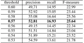
Table 4: F-measure calculated by cross-validation within the training data for each threshold in “intermediate-similarity cluster”
threshold precision recall F-measure
0.60 49,71 14.95 22.99
0.59 52.92 15.05 23.44
0.58 55.08 16.64 25.56
0.57 52.81 16.93 25.64
0.56 49.15 14.45 22.34
0.55 51.51 14.84 23.04
0.54 51.89 15.21 23.52
0.53 54.59 13.61 21.78
As an example, we show the table of obtained ineffective feature types for one fold of cross-validation (Table 3). The threshold was set to 0.90 in this fold.
4.1.2 Threshold between intermediate- and low-similarity clusters
We will next explain how to estimate the threshold between intermediate- and low-similarity clusters.
There are numerous no-relation pairs in low-similarity pairs. We expected that this imbalance would adversely affect classification. We therefore simply attemted to exclude low-similarity pairs. We decreased the threshold by 0.01 from the threshold between high- and intermediate-similarity clusters. We chose a value that yielded the best average F-measure calculated by the cross-validation within the training data. The average value of the thresh-old was 0.57. Table 4 is an example of threshthresh-olds and F-measures for one fold.
4.2 Results of identifying EQ pairs
The results of EQ identification are shown in Ta-ble 5. We tested the following models:
Bow-cos: This is the simplest baseline we used. We represented
sentences with bag-of-words model. Instances with the cosine similarity in Eq. (1) larger than a threshold were classified as
Table 5: Results of identifying EQ pairs
precision recall F-measure
Bow-cos 87.29 57.35 69.22
basic features
Clusterwise 81.98 59.40 68.88 Non-Clusterwise 86.10 59.49 70.36 ClusterC2F 94.96 62.27 75.22
with additional features
Clusterwise 80.93 59.74 68.63 Non-Clusterwise 86.11 60.16 70.84 ClusterC2F 94.99 62.65 75.50
Table 6: Results with basic features
Results for “high-similarity cluster” precision recall F-measure Clusterwise 94.23 96.83 95.51 Non-clusterwise 95.51 96.29 95.90 ClusterC2F 94.23 96.83 95.51 Results for “intermediate-similarity cluster” Clusterwise 42.77 23.03 29.94 Non-clusterwise 53.46 25.31 34.36 ClusterC2F 100.00 36.29 53.25
data was chosen.
Non-Clusterwise: This is a supervised method without the
clusterwise approach. One classifier was constructed regard-less of the similarity of the instance. We used the second degree polynomial kernel. Soft margin parameterCwas set to 0.01.
Clusterwise: This is a clusterwise method without the
coarse-to-fine approach. The second degree polynomial kernel was used. Soft margin parameterCwas set to 0.1 for high-similarity cluster and 0.01 for the other clusters.
ClusterC2F: This is our model, which integrates clusterwise
classification with the coarse-to-fine approach (Figure 1).
Table 5 shows that ClusterC2F yielded the best F-measure regardless of presence of additional fea-tures. The difference between ClusterC2F and the others was statistically significant in the Wilcoxon signed rank sum test with 5% significance level.
4.3 Results for each cluster
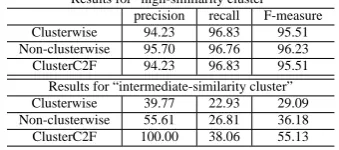
We examined the results for each cluster. The re-sults with basic features are summarized in Table 6 and those with basic features plus additional fea-tures are in Table 7. The tables show that there are no significant differences among the models for high-similarity cluster. However, there are sig-nificant differences for intermediate-similarity clus-ter. We thus concluded that the proposed model (ClusterC2F) works especially well in intermediate-similarity cluster.
Table 7: Results with additional features
Results for “high-similarity cluster” precision recall F-measure Clusterwise 94.23 96.83 95.51 Non-clusterwise 95.70 96.76 96.23 ClusterC2F 94.23 96.83 95.51 Results for “intermediate-similarity cluster” Clusterwise 39.77 22.93 29.09 Non-clusterwise 55.61 26.81 36.18 ClusterC2F 100.00 38.06 55.13
5 Identification of TR pairs
We regarded the identification of the relations be-tween sentences as binary classification, whether a pair of sentences is classified into TR or not. We used SVMs (Vapnik, 1998).
The sentence pairs in TR have the same numeric attributes with different values, as mentioned in In-troduction. Therefore, VNPs will be good clues for the identification.
5.1 Extraction of VNPs
We extract VNPs in the following way.
1. Search for noun phrases that have numeric ex-pressions (we call them numeric phrases).
2. Search for the phrases that the numeric phrases depend on (we call them predicate phrases). 3. Search for the noun phrases that depend on the predicate phrases.
4. Extract the noun phrases that depend on the noun phrases found in step 3, except for date expres-sions. Both the extracted noun phrases and the noun phrases found in step 3 were regarded as VNPs.
In the example in Introduction, “one million” and “1,500,000” are numeric phrases, and “had reached” is a predicate phrase. Then, “the number of users of its mobile-phone service” is a VNP.
5.2 Features for identifying TR pairs
We used some features used in EQ identification: sentence-level uni-, bi-, tirgrams, and bunsetsu-chunk unigrams, normalized lengths of sentences, difference in publication dates, position of sentences in documents, semantic similarities, conjunctions, expressions at the end of sentences, and named enti-ties. In addition, we use the following features.
ands2 is used. If there are more than one VNP, the
largest cosine similarity is chosen.
2. Similarities through bigrams and trigrams in VNPs: These features are defined similarly to the previous feature, but each VNP is represented by the frequency vector of word bi- and trigrams.
3. Similarities of noun phrases in nominative case: Instances in TR often have similar subjects. A noun phrase containing a ga-, wa-, or mo-case is regarded as the subject phrase of a sentence. The similarity is calculated by Eq. (1) with the frequency vectors of nouns in the phrase.
4. Changes in value of numeric attributes: This fea-ture is 1 if the values of the numeric phrases in the two sentences are different, otherwise 0.
5. Presence of numerical units: If a numerical unit is present in both sentences, the value of the feature is 1, otherwise 0.
6. Expressions that mean changes in value: In-stances in TR often contain those expressions, such as ‘reduce’ and ‘increase’ (Nanba et al., 2005). We have three features for each of these expressions. The first feature is 1 if both sentences have the ex-pression, otherwise 0. The second is 1 ifs1 has the
expression, otherwise 0. The third is 1 ifs2 has the
expression, otherwise 0.
7. Predicates: We define one feature for a predicate. The value of this feature is 1 if the predicate appears in the two sentences, otherwise 0.
8. Reporter: This feature represents who is report-ing the incident. This feature is represented by the cosine similarity between the frequency vectors of nouns in phrases respectively expressing reporters in s1ands2. The subjects of verbs such as ‘report’ and
‘announce’ are regarded as phrases of the reporter.
5.3 Use of EQ
A pair of sentences in TR often has a high degree of similarity. Such pairs are likely to be confused with pairs in EQ. We used the identified EQ pairs for the identification of TR in order to circumvent this confusion. Pairs classified as EQ with our method were excluded from candidates for TR.
Table 8: Results of identifying TR pairs
precision recall F-measure
Bow-cos 27.44 41.26 32.96
NANBA 19.85 45.96 27.73
WithoutEq 42.41 47.06 44.61
WithEq 43.13 48.51 45.67
WithEqActual 43.06 48.55 45.64
6 Experiments on identifying TR pairs
Most experimental settings are the same as in the ex-periments of EQ identification. Sentence pairs with-out numeric expressions were excluded in advance and 55,547 pairs were left. This exclusion process does not degrade recall at all, because TR pairs by
definition contain numberic expressions.
We used precision, recall and F-measure for eval-uation. We employed 10-fold cross validation.
6.1 Results of identifying TR pairs
The results of the experiments are summarized in Table 8. We compared four following models with ours. A linear kernel was used in SVMs and soft margin parameterCwas set to 1.0 for all models:
Bow-cos (baseline): We calculated the similarity through
VPNs. If the similarity was larger than a threshold and the two
sentences had the same expressions meaning changes in value and had different values, then this pair was classified as TR. The threshold was set to 0.7, which yielded the best F-measure in the test data.
NANBA (Nanba et al., 2005): If the unigram cosine similarity
between the two sentences was larger than a threshold and the two sentences had expressions meaning changes in value, then this pair was classified as TR. The value of the threshold was set to 0.42, which yielded the best F-measure in the test data.
WithEq (Our method): This model uses the identified EQ
pairs.
WithoutEq: This model uses no information on EQ.
WithEqActual: This model uses the actual EQ pairs given by
oracle.
The results in Table 8 show that bow-cos is better than NANBA in F-measure. This result suggests that focusing on VNPs is more effective than a simple bag-of-words approach.
WithEq and WithEqActual were better than With-outEq. This suggests that we successfully excluded
EQ pairs, which are TR look-alikes. WithEq and
to improve the identification of TR pairs.
7 Conclusion
We proposed methods for identifying EQ and TR pairs in different newspaper articles on an event. We empirically demonstrated that the methods work well in this task.
Although we focused on resolving a bias in the dataset, we can expect that the classification perfor-mance will improve by making use of methods de-veloped in different but related tasks such as Textual Entailment recognition on top of our method.
References
Ido Dagan, Oren Glickman, and Bernardo Magnini. 2005. The pascal recognising textual entailment chal-lenge. In Proceedings of the PASCAL Challenges Workshop on Recognising Textual Entailment, pages 177–190.
Harold Edmundson. 1969. New methods in automatic extracting. Journal of ACM, 16(2):246–285.
Junji Etoh and Manabu Okumura. 2005. Making cross-document relationship between sentences cor-pus. In Proceedings of the Eleventh Annual Meeting of the Association for Natural Language Processing (in Japanese), pages 482–485.
Mamiko Hatayama, Yoshihiro Matsuo, and Satoshi Shi-rai. 2001. Summarizing newspaper articles using ex-tracted information and functional words. In 6th Natu-ral Language Processing Pacific Rim Symposium (NL-PRS2001), pages 593–600.
Vasileios Hatzivassiloglou, Judith L. Klavans, and Eleazar Eskin. 1999. Detecting text similarity over short passages: Exploring linguistic feature combi-nations via machine learning. In Proceedings of the Empirical Methods for Natural Language Processing, pages 203–212.
Vasileios Hatzivassiloglou, Judith L. Klavans, Melissa L. Holcombe, Regina Barzilay, Min-Yen Kan, and Kath-leen R. McKeown. 2001. Simfinder: A flexible clus-tering tool for summarization. In Proceedings of the Workshop on Automatic Summarization, pages 41–49.
Satoru Ikehara, Masahiro Miyazaki, Satoshi Shirai, Akio Yokoo, Hiromi Nakaiwa, Kentaro Ogura, Yoshifumi Oyama, and Yoshihiko Hayashi. 1997. Goi-Taikei – A Japanese Lexicon (in Japanese). Iwanami Shoten.
Tsuneaki Kato, Mitsunori Matsushita, and Noriko Kando. 2005. Must:a workshop on multimodal sum-marization for trend information. In Proceedings of the NTCIR-5 Workshop Meeting, pages 556–563.
William Mann and Sandra Thompson. 1987. Rhetorical structure theory: Description and construction of text structures. In Gerard Kempen, editor, Natural Lan-guage Generation: New Results in Artificial Intelli-gence, Psychology, and Linguistics, pages 85–96. Ni-jhoff, Dordrecht.
Daniel Marcu and Abdessamad Echihabi. 2002. An unsupervised approach to recognizing discourse rela-tions. In Proceedings of the 40th Annual Meeting of the Association for Computational Linguistics, pages 368–375.
Daniel Marcu. 2000. The rhetorical parsing of un-restricted texts a surface-based approach. Computa-tional Linguistics, 26(3):395–448.
Hidetsugu Nanba, Yoshinobu Kunimasa, Shiho Fukushima, Teruaki Aizawa, and Manabu Oku-mura. 2005. Extraction and visualization of trend information based on the cross-document structure. In Information Processing Society of Japan, Special Interest Group on Natural Language Processing (IPSJ-SIGNL), NL-168 (in Japanese), pages 67–74.
Manabu Okumura, Takahiro Fukushima, and Hidetsugu Nanba. 2003. Text summarization challenge 2 -text summarization evaluation at ntcir workshop 3. In HLT-NAACL 2003 Workshop: Text Summarization (DUC03), pages 49–56.
Dragomir Radev. 2000. A common theory of infor-mation fusion from multiple text sources, step one: Cross-document structure. In Proceedings of the 1st ACL SIGDIAL Workshop on Discourse and Dialogue, pages 74–83.
Azriel Rosenfeld and Gorden Vanderbrug. 1977. Coarse-fine template matching. IEEE transactions Systems, Man, and Cybernetics, 7:104–107.
Gorden Vanderburg and Azriel Rosenfeld. 1977. Two-stage template matching. IEEE transactions on com-puters, 26(4):384–393.
Vladimir Vapnik. 1998. Statistical Learning Theory. John Wiley, New York.
Kenji Yokoyama, Hidetsugu Nanba, and Manabu Oku-mura. 2003. Discourse analysis using support vector machine. In Information Processing Society of Japan, Special Interest Group on Natural Language Process-ing (IPSJ-SIGNL), 2003-NL-155 (in Japanese), pages 193–200.