Multi-objective Graph Mining Algorithms for Detecting and Predicting Communities in Complex Dynamic Networks.

(1)

ABSTRACT

BELLO LANDER, GONZALO ALEJANDRO. Multi-objective Graph Mining Algorithms for Detecting and Predicting Communities in Complex Dynamic Networks. (Under the direction of Nagiza F. Samatova.)

Mining patterns in real-world systems represented as complex networks is a key task in many scientific domains. Most graph mining algorithms identify patterns that satisfy a single criterion, which is usually related to the structure of the graph. However, complex networks inherently have multiple sources of information. First, there is often a phenomenon of interest related to the underlying system that we want to analyze or predict, such as a particular phenotype in biological networks or a weather event in climate networks. Second, vertices in complex networks often have attributes that characterize them, such as age or gender in social networks or research area in citation networks. Moreover, complex networks are often dynamic in nature; that is, they change over time. Thus, identifying “interesting” patterns in complex networks often requires looking beyond the structure of the graph by incorporating additional sources of information, such as vertex attributes or a response variable of interest, and addressing the dynamic nature of the network.

Therefore, we posit that the emphasis of graph mining research should shift from the tra-ditional structure-focused approaches to a multi-objective approach that incorporates multiple sources of information. In practice, this translates to a move from single-objective graph mining algorithms to multi-objective algorithms that identify patterns by optimizing multiple objec-tive functions simultaneously while also taking into account the dynamic nature of the network. In this dissertation, we illustrate the value of this multi-objective approach in the context of community detection, an essential graph mining task.

First, we propose a multi-objective algorithm to detect communities associated with a re-sponse variable of interest. We applied our proposed algorithm to identify communities in climate networks associated with seasonal rainfall variability. The results obtained suggest that our algorithm is able to capture the underlying patterns known to be associated with the phe-nomenon of interest and to identify communities with greater predictive power for the response variable than state-of-the-art single-objective algorithms.

(2)

(3)

(4)

Multi-objective Graph Mining Algorithms for Detecting and Predicting Communities in Complex Dynamic Networks

by

Gonzalo Alejandro Bello Lander

A dissertation submitted to the Graduate Faculty of North Carolina State University

in partial fulfillment of the requirements for the Degree of

Doctor of Philosophy

Computer Science

Raleigh, North Carolina

2017

APPROVED BY:

Dennis R. Bahler Rada Y. Chirkova

R. Raju Vatsavai Nagiza F. Samatova

(5)

DEDICATION

A mis padres, Iraida y Gonzalo, por su amor y apoyo incondicional.

(6)

BIOGRAPHY

(7)

ACKNOWLEDGEMENTS

First and foremost, I would like to thank my advisor, Dr. Nagiza F. Samatova, for her constant guidance throughout my graduate studies. Her invaluable advice and the numerous opportuni-ties she provided for my professional development have allowed me to grow as an individual, a researcher, and a future professor.

I would also like to thank the faculty at North Carolina State University’s Department of Computer Science, particularly the members of my advisory committee–Dr. Dennis R. Bahler, Dr. Rada Y. Chirkova, and Dr. R. Raju Vatsavai–for their time and insightful suggestions regarding this dissertation, and Dr. George N. Rouskas, Director of Graduate Programs, for his help and assistance.

I am also grateful to my collaborators from the National Science Foundation (NSF) Ex-peditions in Computing project “Understanding Climate Change: A Data Driven Approach,” particularly Dr. Fredrick H. M. Semazzi at North Carolina State University’s Department of Marine, Earth, and Atmospheric Sciences (MEAS) and Dr. Vipin Kumar at the University of Minnesota. The work I performed as part of this project constitutes an integral part of this dissertation. I am very thankful to Dr. Semazzi’s research group, particularly to Michael Angus and Dr. Pascal F. Waniha, for their useful input regarding the application of my work in the climate science domain.

I would like to thank my fellow students and collaborators at Dr. Samatova’s research group for their many contributions to my work, particularly Steve Harenberg and also Mandar S. Chaudhary, Jitendra K. Harlalka, Stephen Ranshous, Navya Pedemane, Abhishek Agrawal, David “Drew” Boyuka, Lucia Gjeltema, Doel L. Gonzalez, and Kanchana Padmanabhan.

I am especially thankful to my dear friend, Asad Rahman, for constantly pushing me to succeed and achieve my goals.

Finally, I would like to thank my family, particularly my parents, Iraida and Gonzalo, and my grandmother, Consuelo. Without their unconditional love and support, this dissertation would not have been possible.

(8)

TABLE OF CONTENTS

List of Tables . . . vii

List of Figures . . . ix

Chapter 1 Introduction . . . 1

1.1 Introduction . . . 1

1.2 Community Detection . . . 2

1.3 Multi-Objective Community Detection . . . 3

1.3.1 Detecting Communities Associated with a Response Variable . . . 5

1.3.2 Detecting Communities in Dynamic Attributed Graphs . . . 6

1.3.3 Predicting Future Communities in Dynamic Graphs . . . 6

Chapter 2 Detecting Communities Associated with a Response Variable of Interest . . . 8

2.2 Problem Statement . . . 10

2.3 Response-Guided Community Detection . . . 11

2.3.1 Greedy Algorithm for Response-Guided Community Detection . . . 12

2.3.2 Simulated Annealing for Response-Guided Community Detection . . . 13

2.4 Climate Index Discovery . . . 15

2.5 Response-Guided Network Construction . . . 17

2.5.1 Selecting the Set of Vertices . . . 17

2.5.2 Defining the Set of Edges . . . 18

2.5.3 Incorporating Spatial Neighborhood Information and Multiple Related Response Variables . . . 18

2.6 Experimental Evaluation . . . 19

2.6.1 Data Description . . . 20

2.6.2 Data Preprocessing . . . 20

2.6.3 Climate Networks Constructed . . . 21

2.6.4 Climate Indices Discovered . . . 22

2.6.5 Seasonal Rainfall Prediction . . . 24

2.6.6 Physical Interpretation of Climate Indices Discovered . . . 27

2.7 Conclusion . . . 28

Chapter 3 Detecting Communities in Dynamic Attributed Graphs . . . 29

3.2 Related Work . . . 30

3.4 Community Detection in Dynamic Attributed Graphs . . . 31

3.4.1 Measuring the Quality of the Partition of the Graph . . . 31

3.4.2 Detecting Communities in Attributed Graphs . . . 33

3.4.3 Updating Communities in Dynamic Graphs . . . 35

(9)

3.4.5 Generating Benchmark Dynamic Attributed Graphs . . . 37

3.5.1 Benchmark Graphs . . . 38

3.5.2 Real-World Networks . . . 44

Chapter 4 Predicting Future Communities in Dynamic Graphs . . . 51

4.2 Related Work . . . 52

4.4 Hypothesis . . . 53

4.4.1 Data . . . 53

4.4.2 Evaluation . . . 53

4.5 Community Prediction in Dynamic Graphs . . . 55

4.5.1 Computing Edge Likelihoods . . . 57

4.5.2 Detecting Communities . . . 59

4.6.1 Synthetic Graphs . . . 61

4.6.2 Real-World Networks . . . 64

Chapter 5 Conclusion . . . 70

5.2 Future Work . . . 71

(10)

LIST OF TABLES

Table 2.1 Properties of networks constructed and climate indices discovered for OND rainfall variability in the GHA, using the proposed, baseline, and state-of-the-art (SOTA) [57] methodologies with the Louvain method (LM), simu-lated annealing (SA) and Walktrap as the community detection algorithms: number of networks (Num Nets), average number of vertices and edges per network (Avg Vtxs, Avg Edges), average modularity (Avg Mod), number of indices (Num Idxs), average number of vertices, standard deviation, and internal density per index (Avg Vtxs, Avg Std, Avg Dens), and percentage of indices with a statistically significant (p <0.01) linear correlation with the response variable of interest (% Idxs). Best values are highlighted in bold. . . 23 Table 2.2 Average linear correlation with OND rainfall at each station and at the

GHA region, over the training set and the test set, of climate indices discov-ered for OND rainfall variability in the GHA using the proposed, baseline, and state-of-the-art (SOTA) [57] methodologies with the Louvain method (LM), simulated annealing (SA) and Walktrap as the community detec-tion algorithms. Check marks (X) indicate that our proposed methodology performs significantly better according to a two-way ANOVA with a sig-nificance level of 0.05. Best values are highlighted in bold. . . 24 Table 2.3 Linear correlation between true and predicted rainfall (Corr) and RMSE

scores for predictions of OND rainfall at each station and at the GHA re-gion from 1998 to 2011 obtained using the proposed, baseline, and state-of-the-art (SOTA) [57] methodologies with the Louvain method (LM), simu-lated annealing (SA) and Walktrap as the community detection algorithms. Check marks (X) indicate that our proposed methodology performs sig-nificantly better according to a two-way ANOVA with a significance level of 0.05. Best values are highlighted in bold. . . 25

Table 3.1 Number of vertices and number of edges per time step of real-world networks 45 Table 3.2 Results obtained (number of communities, modularity, average density,

(11)

Table 3.3 Number of vertices (Num Vertices), percentage of vertices from previous time step (% t−1 Vertices), and top 3 attributes per time step for the largest community in the DBLP network att= 0, illustrating the evolution of this community fromt= 0 to t= 7. Attributes in the DBLP network, such as Computer Science (CS), Math, Systems, Engineering (Eng), and Artificial Intelligence (AI), represent authors’ areas of publication. . . 49

(12)

LIST OF FIGURES

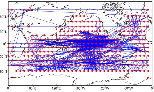
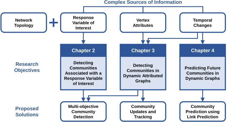
Figure 1.1 Example of a climate network constructed using monthly sea surface tem-perature data from 2000 to 2010. Vertices (red circles) correspond to spa-tial points in a global grid and edges (blue lines) indicate statistically significant correlations between the underlying sea surface temperature data at a pair of spatial points. . . 2 Figure 1.2 Overview of the dissertation. In Chapter 2, we propose a multi-objective

algorithm to detect communities associated with a response variable of interest. In Chapter 3, we propose a multi-objective algorithm to detect, update, and track communities in dynamic attributed graphs. In Chap-ter 4, we propose a methodology to predict future communities in dynamic graphs using link prediction methods. . . 5

Figure 2.1 Overview of the proposed methodology for climate index discovery using response-guided community detection . . . 16 Figure 2.2 Map highlighting (in red) the North Eastern Highlands of Tanzania (left)

and the four stations located in this region that were used for this study: Arusha, Kilimanjaro, Moshi, and Same (right) . . . 20 Figure 2.3 Spatial points selected in the month of October to construct the climate

network. Blue triangles indicate spatial points selected only for individual stations and red circles indicate spatial points in the consensus set. . . 21 Figure 2.4 Climate indices discovered using the proposed methodology with the

multi-objective algorithms for response-guided community detection based on the Louvain method (left) and simulated annealing (right) and with OND rainfall variability in the GHA as the response variable of interest. Each color represents a different index and diamonds indicate overlaps between indices. To improve visualization, only the top 10 indices with the highest association with the response variable over the training set are shown in each figure. . . 22 Figure 2.5 Average linear correlation between true and predicted rainfall for

predic-tions of OND rainfall at each station in the GHA region over the train-ing set ustrain-ing the proposed, baseline, and state-of-the-art (SOTA) [57] methodologies with the Louvain method (LM), simulated annealing (SA) and Walktrap as the community detection algorithms vs. the number of predictors used to build the regression models. The dashed line indicates the number of predictors selected for further analysis. . . 25 Figure 2.6 Linear correlation between true and predicted rainfall and RMSE scores

(13)

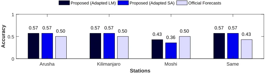
Figure 2.7 Classification accuracy of the prediction of the OND rainfall season at each station in the GHA region from 1998 to 2011 obtained using the proposed methodology with the multi-objective algorithms for response-guided community detection based on the Louvain method (LM) and simulated annealing (SA), as well as official forecasts issued by the TMA . 27 Figure 2.8 Time series of the Ni˜no 3.4 index (upper, solid line) and the IOD index

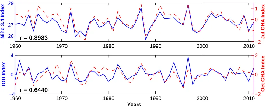
(lower, solid line) with climate indices discovered in July (upper, dashed line) and October (lower, dashed line) using the proposed methodology with the multi-objective algorithm for response-guided community de-tection based on the Louvain method and with OND rainfall variability in the GHA as the response variable of interest. The linear correlation between the time series is shown in the lower left corner of each figure. . . 28

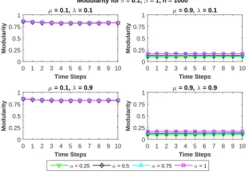
Figure 3.1 Average modularity of the partitions obtained at each time step of the benchmark graphs using our proposed algorithm with update parame-ter β = 1 and multiple values of the weighting parameter α. Bench-mark graphs were generated using the following parameters: number of vertices n = 1000, mixing parameter µ = {0.1,0.9}, noise parameter λ={0.1,0.9}, and change parameterδ = 0.1. . . 39 Figure 3.2 Average attribute similarity of the partitions obtained at each time step

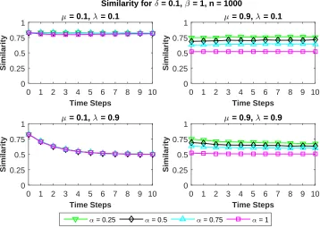
of the benchmark graphs using our proposed algorithm with update pa-rameterβ = 1 and multiple values of the weighting parameterα. Bench-mark graphs were generated using the following parameters: number of vertices n = 1000, mixing parameter µ = {0.1,0.9}, noise parameter λ={0.1,0.9}, and change parameterδ = 0.1. . . 40 Figure 3.3 Average running time (in seconds) at each time step of the benchmark

graphs of our proposed algorithm with weighting parameter α= 0.5 and multiple values of the update parameterβ. Benchmark graphs were gener-ated using the following parameters: number of verticesn={1000,10000}, mixing parameter µ= 0.1, noise parameterλ= 0.1, and change parame-ter δ={0.1,0.9}. . . 41 Figure 3.4 Averagemodularity andattribute similarity of the partitions obtained at

each time step of the benchmark graphs using our proposed algorithm with weighting parameter α = 0.5 and multiple values of the update parameter β. Benchmark graphs were generated using the following pa-rameters: number of vertices n= 1000, mixing parameter µ= 0.1, noise parameter λ = 0.1, and change parameter δ = {0.1,0.9}. Comparable results were obtained for n= 10000. . . 42 Figure 3.5 Box plots of estimated mixing parameter (left) and estimated change

(14)

Figure 3.6 Histogram of vertex change scores (left axis) and probability density func-tions of the two components of a Gaussian mixture model fitted to the vertex change scores using the Expectation Maximization (EM) algorithm (right axis) for benchmark graphs with n= 1000 vertices and change pa-rameter δ = 0.1 (a), 0.5 (b), and 0.9 (c). The corresponding Bayesian information criterion (BIC) values are shown in the upper corner of each figure. Comparable results were obtained for other values of δ. . . 43 Figure 3.7 Average modularity and attribute similarity of the partitions obtained

and averagerunning time (in seconds) at each time step of the benchmark graphs using our proposed algorithm with weighting parameter α = 0.5 and update parameter β = 0.5. Benchmark graphs were generated using the following parameters: number of verticesn= 1000, mixing parameter µ= 0.1, noise parameterλ= 0.1, and change parameter δ= 0.1. . . 44 Figure 3.8 Running time (left, in seconds) andpeak memory(right, in MB) obtained

at each time step of the real-world networks using our proposed algorithm, CODICIL [48], and I-Louvain [11]. Line styles and colors are used to denote the algorithms and marker types are used to denote the data sets. Missing results indicate that the implementation of the algorithm did not run in the allotted time of 5 hours or with the allotted memory of 64GB. 48 Figure 3.9 Word clouds of attributes per time step for the largest community in the

DBLP network att= 0, illustrating the evolution of this community from t= 0 to t= 7. Attributes in the DBLP network, such as Math, Systems, Engineering, and Artificial Intelligence (AI), represent authors’ areas of publication. The Computer Science attribute was omitted from the word clouds as it is the top 1 attribute in all communities. . . 49

Figure 4.1 Baseline Adjusted Rand Index (ARI) obtained on N = 100 synthetic dynamic graphs with δ = 0.1 and various values of µ (left) and with µ= 0.5 and various values of δ (right), where µis the mixing parameter of the graph andδis the percentage of new edges inserted. Shaded regions indicate plus or minus one standard deviation centered around the mean. 54 Figure 4.2 Predicted and baseline Adjusted Rand Index (ARI) obtained onN = 100

synthetic dynamic graphs withµ= 0.5 andδ= 0.1, whereµis the mixing parameter of the graph and δ is the percentage of new edges inserted, for various percentages of edges predicted correctly (left) and incorrectly (right). Shaded regions indicate plus or minus one standard deviation centered around the mean. . . 55 Figure 4.3 State-of-the-art (SOTA) and baseline Adjusted Rand Index (ARI, left)

(15)

Figure 4.4 Adjusted Rand Index (ARI) obtained using the baseline and the proposed community prediction methodology with multiple link prediction meth-ods (Common Neighbors, Jaccard’s Coefficient, Adamic-Adar, Resource Allocation, Katz, and Structural Perturbation Method) on N = 100 syn-thetic dynamic graphs with δ = 0.1 and various values of µ, where µ is the mixing parameter of the graph and δ is the percentage of new edges inserted. Red boxes indicate a statistically significant (p <0.01) improve-ment with respect to the baseline. Comparable results were obtained for other values of δ. . . 62 Figure 4.5 Percentage of edges predicted correctly obtained using multiple link

pre-diction methods (Common Neighbors, Jaccard’s Coefficient, Adamic-Adar, Resource Allocation, Katz, and Structural Perturbation Method) onN = 100 synthetic dynamic graphs withδ = 0.1 and various values ofµ, where µ is the mixing parameter of the graph and δ is the percentage of new edges inserted. Comparable results were obtained for other values of δ. . . 63 Figure 4.6 Adjusted Rand Index (ARI) obtained using the baseline and a

modi-fied version of the proposed community prediction methodology that uses predicted future edges instead of edge likelihoods on N = 100 synthetic dynamic graphs with µ= 0.5 andδ = 0.1, whereµis the mixing parame-ter of the graph and δ is the percentage of new edges inserted. Red boxes indicate a statistically significant (p <0.01) improvement with respect to the baseline. Comparable results were obtained for other values of µ. . . . 64 Figure 4.7 Median number of common neighbors between vertices incident to edges

present at the initial time step t (left) and incident to edges inserted at the following time stept+ 1 (right) onN = 100 synthetic dynamic graphs with δ= 0.1 and various values ofµ, whereµ is the mixing parameter of the graph and δ is the percentage of new edges inserted. Shaded regions indicate plus or minus one standard deviation centered around the mean. 64 Figure 4.8 Predicted and baseline Adjusted Rand Index (ARI) obtained for various

percentages of edges predicted correctly (20%, 40%, 60%, and 80%) on dynamic graphs constructed from real-world data sets: DBLP (left, upper row), TripAdvisor (right, upper row), and Yelp (left, lower row). Shaded regions indicate plus or minus one standard deviation centered around the mean for a sample of size N = 10. . . 66 Figure 4.9 Adjusted Rand Index (ARI, left) and percentage of edges predicted

(16)

(17)

Chapter 1

Introduction

1.1 Introduction

Complex systems across multiple scientific domains are commonly represented as networks, wherevertices correspond to objects in the system andedgescorrespond to interactions between these objects. For example, in biology, the metabolic system can be represented as a network of interacting metabolites [22], while, in climate science, the global climate system can be represented as a network of interacting regions [57] (see Figure 1.1). This representation allows researchers to make use of existing graph mining algorithms to identify “interesting” network patterns, which, in turn, can help them better understand the behavior of the system.

Graph mining algorithms usually identify network patterns in the form of subgraphs that satisfy a given criterion, which, in most cases, is related to the structure of the graph. For ex-ample, maximal clique enumeration algorithms identify complete subgraphs [50], while frequent subgraph mining algorithms identify frequently occurring isomorphic subgraphs [27]. However, given the complex nature of the systems being represented by these networks, identifying “in-teresting” patterns often requires looking beyond the structure of the graph.

On one hand, complex networks inherently have multiple sources of information. For exam-ple, social networks contain not only vertices and edges representing users and their interactions, but also attributes of heterogeneous types (e.g., age, gender) describing these users. However, most graph mining algorithms do not take these additional sources of information into account [1]. In Chapter 2 and Chapter 3, we show that incorporating additional sources of information, such as vertex attributes or a response variable of interest, allows us to identify more meaningful patterns.

(18)

Figure 1.1: Example of a climate network constructed using monthly sea surface temperature data from 2000 to 2010. Vertices (red circles) correspond to spatial points in a global grid and edges (blue lines) indicate statistically significant correlations between the underlying sea surface temperature data at a pair of spatial points.

of the network [1]. In Chapter 3, we show that incorporating the temporal changes of the net-work allows us to identify patterns more efficiently. Furthermore, in Chapter 4, we show that this also allows us to predict these patterns in future time steps.

For these reasons, we posit that the emphasis of graph mining research should shift from the traditional structure-focused approaches to a multi-objective approach that incorporates multiple sources of information in addition to the structural properties of the graph. In practice, this translates to a move from single-objective graph mining algorithms to multi-objective algorithms that identify patterns by optimizing multiple objective functions simultaneously while also taking into account the dynamic nature of the network. In this dissertation, we illustrate the value of this multi-objective approach in the context of one specific graph mining task: community detection.

1.2 Community Detection

(19)

patterns in climate networks [57].

Identifying the community structure of a network is essential for understanding the underly-ing system. Therefore, community detection has become one of the most important tasks in the field of network analysis [18, 23], with applications in many domains. Most existing methods for community detection partition the network into a set of communities C by optimizing a single objective function f, which typically measures some structural property of the graph; that is,

min

C∈Ωf(C) (1.1)

where Ω is the set of feasible solutions.

While no objective function for community detection is universally accepted [18], the goal of most existing methods is to optimize the trade-off between the intra-cluster density and the cluster density of the communities identified. The intra-cluster density and the inter-cluster density of a community ci,Dint(ci) and Dext(ci), respectively, are given by

Dint(ci) =

kintci 1

2 · |ci|(|ci| −1)

(1.2)

Dext(ci) = kextci |ci|(n− |ci|)

(1.3)

wherekintci is the number of edges between vertices in communityci (i.e., internal edges),kextci

is the number of edges between vertices in communityciand the rest of the graph (i.e., external edges), andn is the number of vertices in the graph.

However, as is the case with graph mining in general, this single-objective approach to com-munity detection may be insufficient because it limits the communities identified to those that satisfy a particular structural property. This is especially true when the structural information of the network is incomplete or noisy (i.e., missing or incorrect edges). In these cases, incorpo-rating additional sources of information, such as vertex attributes, would allow us to identify the community structure of the network more precisely [64]. For this reason, we posit that a shift towards multi-objective community detection methods that take into account multiple sources of information simultaneously is needed.

1.3 Multi-Objective Community Detection

Multi-objective community detection methods partition a network into a set of communitiesC by optimizing multiple objective functions simultaneously; that is,

min

(20)

where Ω is the set of feasible solutions andfi(C) fori= 1,2, ..., kare the objective functions. A solution to Equation 1.4 is said to bePareto optimal if it is not possible to modify this solution to improve at least one of the objective functions without degrading any of the rest [51].

Multi-objective community detection has been recently proposed as a means to incorporate multiple structural properties of the graph into the community detection process [52, 51, 63]. For example, Shi et al. [52, 51] and Wu and Pan [63] make use of evolutionary algorithms to identify communities by optimizing two objective functions that measure the intra-cluster density and the inter-cluster density, respectively.

In this dissertation, we further capitalize on the concept of multi-objective community de-tection by incorporating not only the structural properties of the graph, but also additional sources of information, such as vertex attributes or a response variable of interest, while taking into account the dynamic nature of the network. Our general approach is to optimize multiple objective functions that measure these different sources of information using the well-known weighted sum method [41]; that is, we optimize a linear combination of the multiple objective functions given by

min C∈Ω

k

X

i=1

wifi(C) (1.5)

where Ω is the set of feasible solutions, fi(C) for i = 1,2, ..., k are the objective functions, and wi fori= 1,2, ..., k are weighting parameters that denote the relative importance of each objective function. A solution to Equation 1.5 is Pareto optimal ifwi>0 fori= 1,2, ..., k[54]. Moreover, if the graphs are dynamic, we also incorporate the temporal changes of the different sources of information in order to update the communities more efficiently or to predict the communities in future time steps.

It is worth noting that evolutionary algorithms for multi-objective optimization, such as the ones used in previous studies [52, 51, 63], have certain advantages over the weighted sum method: they do not require weighting parameters and they allow us to identify a set of Pareto optimal solutions instead of a single Pareto optimal solution. However, evolutionary algorithms are computationally expensive, and thus they are not suitable for the large-scale networks in most real-world applications.

We adopt this multi-objective approach to tackle three distinct research objectives related to community detection in complex networks:

Detecting communities associated with a response variable of interest that can be used to analyze or predict this response variable.

Detecting communities in dynamic attributed graphs.

(21)

These objectives, which correspond to the main chapters of this dissertation (see Figure 1.2), are further explained in the following sections.

Proposed Solutions Research Objectives Community Updates and Tracking Community Prediction using Link Prediction Multi-objective Community Detection Detecting Communities Associated with a Response Variable of Interest Chapter 2 Detecting Communities in Dynamic Attributed Graphs Chapter 3 Predicting Future Communities in Dynamic Graphs Chapter 4

Complex Sources of Information

Response Variable of Interest Vertex Attributes Network Topology Temporal Changes

Figure 1.2: Overview of the dissertation. In Chapter 2, we propose a multi-objective algorithm to detect communities associated with a response variable of interest. In Chapter 3, we propose a multi-objective algorithm to detect, update, and track communities in dynamic attributed graphs. In Chapter 4, we propose a methodology to predict future communities in dynamic graphs using link prediction methods.

1.3.1 Detecting Communities Associated with a Response Variable

Communities in complex networks may be used to analyze or predict a phenomenon of interest related to the system represented by the network. For example, communities in climate networks may be used to predict a weather event [57], while communities in biological networks may be used to analyze a particular disease [24]. However, single-objective community detection algorithms do not take into account the variability of this phenomenon of interest, and thus the communities identified may not necessarily be associated with it.

(22)

summarize spatiotemporal climate patterns–associated with seasonal rainfall variability, a key task in the climate science domain. The results obtained suggest that our proposed algorithm is able to capture the underlying patterns known to be associated with the phenomenon of interest. Moreover, the communities identified using our proposed algorithm were shown to have a greater predictive power for the response variable than communities identified using single-objective algorithms [57].

1.3.2 Detecting Communities in Dynamic Attributed Graphs

Vertices in complex networks usually have individual properties, orattributes, that characterize them, such as age or gender in social networks or research area in citation networks. Moreover, complex networks are oftendynamicin nature; that is, they are constantly changing. While some multi-objective algorithms for community detection in attributed graphs have been recently proposed [11], none of them also identify communities in dynamic graphs, and thus would need to be run from scratch every time the graph changes. Moreover, most of these algorithms are designed to handle only certain attribute types, which hinders their applicability to real-world networks.

For this reason, in Chapter 3 [5], we propose a multi-objective algorithm for community detection in dynamic attributed graphs that incorporates both the structural properties of the graph and the attributes of the vertices while also taking into account the dynamic nature of the network. Our proposed algorithm handles graphs with heterogeneous attribute types, as well as changes to both the structure of the graph and the attribute information of the vertices, which is essential for its applicability to real-world networks. We evaluated our proposed algorithm on a variety of synthetically generated dynamic attributed graphs and on large-scale real-world networks. The results obtained show that our proposed algorithm is able to identify graph partitions with modularity and attribute similarity comparable to that of state-of-the-art algorithms [11, 48]. However, the time and memory requirements of the state-of-the-state-of-the-art algorithms are considerably higher, suggesting that our proposed algorithm is able to achieve a better trade-off between efficiency and quality of the communities identified.

1.3.3 Predicting Future Communities in Dynamic Graphs

(23)

(24)

Chapter 2

Detecting Communities Associated

with a Response Variable of Interest

2.1 Introduction

Detecting communities in complex networks is a key task in many scientific domains, such as climate science and biology. As discussed in Chapter 1, scientists in these domains are often concerned with finding communities associated with aresponse variable of interest that can be used to analyze or predict this response variable. For example, in climate science, such commu-nities may represent spatiotemporal climate patterns associated with a particular weather event (e.g., precipitation) [57], while, in biology, they may represent groups of functionally associated genes associated with a particular disease (e.g., Alzheimer’s disease) [24].

(25)

defined for El Ni˜no Southern Oscillation (ENSO)–one of the most widely studied climate pat-terns, characterized by temperature and pressure anomalies over the Pacific Ocean–are used to forecast Atlantic hurricane activity [20].

Climate indices were traditionally the product of hypothesis-driven research. However, the increasing amount of climate data available has led to the adoption of data-driven approaches to guide and accelerate climate index discovery. The most common of such approaches is the use of Principal Component Analysis (PCA)–known in the climate science domain as Empir-ical Orthogonal Function (EOF) analysis–to identify major modes of variability in the data. However, the use of eigenvalue analysis techniques, such as PCA, to discover climate indices has important limitations with respect to the physical interpretability of the climate indices discovered and the ability of these techniques to detect weaker patterns [55].

An alternative approach to climate index discovery is the application of clustering tech-niques, such as Shared Nearest Neighbor (SNN) clustering, to identify regions of homogeneous long-term variability in climate data [55] or, more recently, the application of community detec-tion methods to identify communities in climate networks [57]. The validity of the clusters or communities identified as climate indices has been evaluated in terms of their ability to predict a response variable of interest, such as temperature or precipitation [55, 57]. However, since none of these methods take the response variable into account, the climate indices discovered may not necessarily be good predictors.

For this reason, we propose a methodology to discover climate indices associated with a re-sponse variable of interest that makes use of a multi-objective community detection algorithm that explicitly incorporates information of this response variable into the community detection process. We apply this methodology to the discovery of climate indices associated with seasonal rainfall variability in the Greater Horn of Africa (GHA) and validate the climate indices dis-covered in terms of their predictive power and climatological relevance. Our results show that discovering climate indices associated with a response variable of interest allows us to identify its potential sources of variability. Moreover, using these climate indices as predictors allows us to improve forecasts of the response variable. This is especially important because improving the accuracy of regional climate forecasts, particularly of precipitation, is one of the major current challenges in climate science [49].

(26)

of multivariate spatiotemporal data that, unlike existing network construction methodologies [56, 57, 61], builds the network in a response-guided manner while also incorporating multiple covariates, spatial neighborhood information, and multiple related response variables into the network construction process (Section 2.5).

The rest of this chapter is organized in the following way. In Section 2.2, we formally de-fine the problem of response-guided community detection. In Section 2.3, we describe a general multi-objective strategy for response-guided community detection and present two examples of community detection algorithms that can be adapted in this way to identify communities asso-ciated with a response variable of interest. We present an overview of our proposed methodology for the discovery of climate indices associated with a response variable of interest in Section 2.4, and detail our proposed network construction methodology in Section 2.5. In Section 2.6, we describe the experimental evaluation of our proposed methodology for climate index discovery and report the results obtained. Finally, we present our conclusions in Section 2.7.

2.2 Problem Statement

Let X = {xt,d,f ∈ R|t ∈ T, d ∈ D, f ∈ F} be a multivariate spatiotemporal data set and

Y ={yt∈R|t∈T}be a response variable, whereT is a set of time steps,D is a set of spatial

points, and F is a set of covariates. For our motivating application of climate index discovery, X may be a global climate data set for a given month, Y may be the total rainfall at a target region for a given season, T may be a set of years, Dmay be a set of global coordinates, and F may be a set of climate variables (e.g., temperature, pressure, humidity).

Let data setX be represented as a graphG= (V, E), whereV ⊆Dis the set of vertices,E is the set of edges, and each edge (d1, d2)∈E is defined based on a domain-specific relationship

between the data at spatial points d1 and d2 for all covariates f ∈ F and over all time steps

t∈T. For our motivating application of climate index discovery, an edge (d1, d2) may represent

a statistically significant correlation between the data at spatial points d1 and d2.

Informally, we defineresponse-guided community detection as the task of partitioning graph Ginto a set of communitiesC, such that every communityci∈Cis stronglyassociatedwith the response variable Y. To quantify this association, we construct anindex for each community.

Definition 2.1 (Index).Given a communityci, the index constructed forci using covariate f ∈F,Ii,f, is given by

Ii,f(t) = 1 |ci|

X

d∈ci

xt,d,f ∀t∈T (2.1)

(27)

Definition 2.2 (Association).Given a communityci, theassociationofci with the response variable Y, φ(ci), is given by

φ(ci) = max

f∈F |rIi,f,Y| (2.2)

where rIi,f,Y is the Pearson’s linear correlation coefficient between index Ii,f and the response variable Y over all time steps t∈T.

Definition 2.3 (Average Association).Given a set of communities C, the average asso-ciation of C with the response variableY,φ¯(C), is given by

¯

φ(C) = 1 |C|

X

ci∈C

φ(ci) (2.3)

where φ(ci) the association of communityci with the response variable Y.

Finally, we formally define the problem of response-guided community detection as follows. Given a graph G = (V, E) and a response variable Y, partition G into a set of communities C ={c1, c2, ..., c|C|}, where

S|C|

i=1ci =V and ci∩cj =∅ for allci, cj ∈C withi6=j, such that the average association of C with the response variableY, ¯φ(C), is maximized.

2.3 Response-Guided Community Detection

A common approach to community detection is to find the set of communities that maximizes a given quality function that measures the “goodness” of the partition of the graph. For tra-ditional community detection, a “good” partition of the graph is generally such that there are many edges within the communities but few edges among them. However, for response-guided community detection, the goal is to identify communities strongly associated with a response variable of interest. Therefore, we must maximize not only the “goodness” of the partition of the graph, but also the association of the communities in the partition with this variable.

To this end, we introduce a multi-objective function,F, given by

F(C) =α·q(C) + (1−α)·φ¯(C) (2.4)

whereC is a set of communities,q(C) is a function of the “goodness” ofC, ¯φ(C) is the average association of the communities in C with the response variable of interest, and α ∈(0,1] is a weighting parameter to balance the trade-off between the “goodness” ofC and the association of the communities with the response variable.

(28)

quality function” for community detection [18]–as the “goodness” function. The modularity of a given partition of a graph is defined as the difference between the number of edges within the communities and the expected number of such edges in a random graph with the same degree distribution [39].

Definition 2.4 (Modularity).LetG= (V, E)be an unweighted, undirected graph partitioned into a set of disjoint communities C ={c1, c2, ..., cK}. The modularity of the partition of G [38] is given by

Q(C) = 1 2m

X

v,w∈V

Avw− kvkw

2m

δ(cv, cw) (2.5)

where A is the adjacency matrix of G (i.e., Avw = 1 if vertices v and w are adjacent and Avw = 0 otherwise), m= 1₂ΣvwAvw is the number of edges in G, kv = ΣwAvw is the degree of vertex v, cv is the community of vertex v, and δ(cv, cw) is the Kronecker delta function (i.e., δ(cv, cw) = 1 if cv =cw and δ(cv, cw) = 0 otherwise).

Maximizing modularity is a computationally hard problem; in fact, the decision version of the modularity maximization problem has been shown to be NP-complete [9]. However, several heuristic algorithms have been proposed to efficiently identify graph partitions with high modularity [18]. A general strategy for response-guided community detection is to adapt these modularity optimization algorithms by replacing modularity with the multi-objective functionF as the optimization criterion. To illustrate this strategy, we present two algorithms that can be adapted in this way to identify communities strongly associated with a response variable of interest: the Louvain method, a greedy algorithm for modularity optimization, and simulated annealing, a probabilistic optimization technique.

2.3.1 Greedy Algorithm for Response-Guided Community Detection

Greedy algorithms for modularity optimization identify communities by iteratively merging ver-tices or communities that result in the largest increase in the modularity of the graph partition [7, 10]. Here, we make use of the Louvain method [7], a well-known, single-objective greedy algorithm for modularity optimization that has been shown to outperform other community detection algorithms in empirical comparative studies [31]. We adapt the Louvain method for response-guided community detection by using the multi-objective function Fas the optimiza-tion criterion. The adapted algorithm (see Algorithm 2.1) proceeds as follows.

(29)

communityci, ∆F(z, ci), is given by

∆F(z, ci) =α·∆Q(z, ci) + (1−α)·∆ ¯φ(z, ci) (2.6)

where ∆Q(z, ci) and ∆ ¯φ(z, ci) are the gain in modularity and the gain in average association with the response variable of interest, respectively.

The gain in modularity resulting from assigning vertex z to community ci, ∆Q(z, ci), can be efficiently computed as follows [7].

∆Q(z, ci) =

"

k0ci+kz,ci

2m −

kci+kz

2m

2# −

"

k0ci

2m −

kci

2m 2 − kz 2m 2#

= kz,ci

2m −

kci·kz

2m2

(2.7)

where kz is the degree of vertexz,kz,ci is the number of edges between vertex z and vertices

in community ci, kci is the number of edges incident to vertices in community ci, k 0

ci is the

number of edges between vertices in communityci, andmis the number of edges in the graph. In the second phase of the algorithm, a new graph is constructed by aggregating the vertices in each community into a single vertex. The number of edges between two vertices in this new graph is given by the sum of the edges between vertices in the two corresponding communities. The first phase of the algorithm is then reapplied on this new graph.

These two phases are repeated iteratively until no further changes to the community struc-ture can be made. Then, the partition that yields the highest value of the multi-objective functionF for the original graph is returned. Note, however, that there is no guarantee of the optimality of the partition. Furthermore, the output of the algorithm depends on the order in which the vertices are iterated over, although empirical analysis indicates that this order does not generally have a significant impact on the value obtained for the objective function [7].

2.3.2 Simulated Annealing for Response-Guided Community Detection Another strategy that has been employed for modularity optimization is simulated annealing [30], an optimization technique that avoids local optima by incorporating stochastic noise into the search procedure. The level of noise is defined by a computational temperature, T, which decreases after each iteration. Here, we adapt the single-objective simulated annealing algorithm proposed by Guimer`a et al. [22] for response-guided community detection by using the multi-objective function Fas the optimization criterion. The adapted algorithm (see Algorithm 2.2) proceeds as follows.

(30)

moving a randomly selected vertex to a randomly selected community. Global moves consist of merging two randomly selected communities and splitting a randomly selected community.

Each local and global move is accepted with probability

p=

  

 

1, if ∆F≥0

exp

∆F T

, if ∆F<0 (2.8)

where ∆Fis the gain in the multi-objective functionF resulting from the local or global move; that is, the gain from moving a vertex z to a community ci, ∆F(z, ci), the gain from merging two communitiesci andcj, ∆F(ci, cj), or the gain from splitting a communityciin two, ∆F(ci). After all local and global moves have been evaluated, the current temperatureT is decreased toT0 =c· T, where c∈(0,1) is a cooling parameter (typically between 0.990 and 0.999). The algorithm stops when a minimum temperature is reached or when there is no change in the multi-objective function Ffor a given number of consecutive iterations.

Algorithm 2.1:Greedy algorithm for response-guided community detection Input : graph,G= (V, E); weighting parameter, α

Output: vector of community memberships, C

1 G0 ←G

2 do

/* Phase one: */

3 for each v∈V do

4 C[v]←v

5 do

6 num moves ← 0

7 for each v∈V do

8 for each communityc_i ∈C connected tov do 9 ∆F(v, ci)←α·∆Q(v, ci) + (1−α)·∆ ¯φ(v, ci) 10 if ∃ci ∈C such that ∆F(v, ci)>0then

11 C[v]←arg max_c

i∈C∆F(v, ci)

12 num moves ← num moves +1

13 while num moves>0

/* Phase two: */

14 Compute the value of the multi-objective function,F(C), forG₀

15 Build a new graphG= (V, E) by aggregating eachc_i ∈C into one vertex 16 while at least one vertex is moved during phase one

(31)

Algorithm 2.2:Simulated annealing algorithm for response-guided community detection Input : graph,G= (V, E); weighting parameter, α; cooling parameter, c; maximum

number of iterations, γ

Output: vector of community memberships, C

1 T ← _|_V2_|

2 num moves ← 0 3 for each v∈V do 4 C[v]←v

5 while T >0 and num moves < γ do

/* Local moves: */

6 fori←1 to |V|2 do

7 Randomly select a vertex v∈V and a community c_i ∈C 8 ∆F(v, ci)←α·∆Q(v, ci) + (1−α)·∆ ¯φ(v, ci)

9 if ∆F(v, c_i)≥0 or random(0,1)≤exp

_∆_F₍_v,c_i) T

then

10 Move v toci

/* Global moves: */

11 fori←1 to |V|do

12 Randomly select two communities ci, cj ∈C

13 ∆F(ci, cj)←α·∆Q(ci, cj) + (1−α)·∆ ¯φ(ci, cj)

14 if ∆F(c_i, c_j)≥0 or random(0,1)≤exp

_∆_F₍_c i,cj) T

then

15 Merge c_i and c_j

16 Randomly select a community c_i∈C 17 ∆F(ci)←α·∆Q(ci) + (1−α)·∆ ¯φ(ci) 18 if ∆F(c_i)≥0 or random(0,1)≤exp

_∆_F₍_c_i) T

then

19 Splitc_i in two communities

20 Compute the value of the multi-objective function,F(C), forG

21 T ←c· T

22 if no move is accepted then 23 num moves ← num moves +1

24 else

25 num moves ← 0

26 return C with the highest value of the multi-objective function,F(C), for G

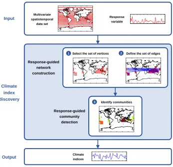
2.4 Climate Index Discovery

(32)

steps (see Figure 2.1). We are given as input a spatiotemporal climate data set and a response variable of interest. First, we represent the multivariate spatiotemporal climate data as a graph using our proposed response-guided network construction methodology (Section 2.5). Second, we identify communities in this graph using one of our adapted algorithms for response-guided community detection (see Section 2.3). For each community ci identified, we return as output an index I_i,f_i∗ potentially associated with the response variable of interest, where f_i∗ is the representative covariate of the community for the response variable, defined as

fi∗ = arg max f∈F

|rIi,f,Y| (2.9)

where rIi,f,Y is the Pearson’s linear correlation coefficient between index Ii,f and the response

variableY over all time stepst∈T.

180oW 120oW 60oW 0o 60oE 120oE 180oW 80o

S 40oS 0o 40oN 80o N Multivariate spatiotemporal data set Response variable Climate indices

180oW 120oW 60oW 0o 60oE 120oE 180oW 80oS

40oS 0o 40oN 80oN

Select the set of vertices

1 2 Define the set of edges

Response-guided network construction Response-guided community detection 3

40oS 0o 40oN 80oN

Identify communities Input Climate index discovery Output

(33)

2.5 Response-Guided Network Construction

Spatiotemporal data can be represented as a graph, where each vertex is a spatial point and each edge indicates a significant relationship between a pair of spatial points. This type of representation has been adopted to model climate data because it captures the dynamical behavior of the climate system [56, 57, 61]. Furthermore, communities in climate networks often have a higher association with the response variable of interest than clusters in climate data obtained using spectral clustering and thek-means clustering algorithm [57]. This shows the potential of community detection methods over traditional clustering techniques as a means for discovering climate indices.

In this chapter, we propose a methodology for the construction of climate networks as-sociated with a response variable of interest from multivariate spatiotemporal data. The key features of this methodology are as follows. First, we construct the network in a response-guided manner. Existing methodologies for climate network construction consider all the spatial points in the data set as vertices and build the network by computing the correlation between every pair of vertices [57, 61]. Given the high-dimensional nature of the data, this can be computa-tionally expensive. In contrast, we only consider as vertices the spatial points associated with the response variable of interest. Second, we incorporate multiple covariates into the network construction process. Some existing methodologies have incorporated multiple covariates by defining a cross correlation function to weight the edges of the network [56]. Here, instead, we use the information of multiple covariates to assess the statistical significance of each edge in the network. Third, we incorporate spatial neighborhood information and multiple related response variables into the network construction process to increase its robustness in the case of data sets with small sample size.

2.5.1 Selecting the Set of Vertices

The set of vertices V of the network is selected based on the statistical significance of the relationship between each spatial point in the data set and the response variable of interest for multiple covariates. To assess this statistical significance, we first calculate the Spearman’s rank correlation coefficients between the time series for each covariate at each spatial point and the response variable. Spearman’s rank correlation is used to capture nonlinear relationships known to exist in climate data [25].

(34)

p-value of the test statistic given by

−2X f∈F

ln(pXd,f,Y) (2.10)

where pXd,f,Y is the p-value of the Spearman’s rank correlation coefficient between the time

series for covariatef at spatial pointd,Xd,f, and the response variableY over all time stepst∈ T. The use of this combined probability test allows us to capture relationships between multiple covariates and the response variable. Finally, the set S of spatial points with a statistically significant combinedp-value (p <0.01) is selected as the set of verticesV of the network. These vertices represent spatial points potentially associated with the response variable of interest.

2.5.2 Defining the Set of Edges

The set of edgesE of the network is defined based on the statistical significance of the relation-ship between each pair of spatial points in V for multiple covariates. To assess this statistical significance, we first calculate the Pearson’s linear correlation coefficients between the time series for each covariate at each pair of spatial points. Despite the presence of nonlinear relationships in climate data, climate networks constructed using Pearson’s linear correlation coefficient have been shown to be highly similar to those constructed using nonlinear measures, such as mutual information [14].

For each pair of spatial points d1, d2 ∈ V, the p-values of the Pearson’s linear correlation

coefficients computed for each covariate are combined using Fisher’s X2 _{test [17]; that is, by}

calculating the p-value of the test statistic given by

−2X f∈F

ln(pXd₁,f,Xd₂,f) (2.11)

wherepXd₁,f,Xd₂,f is thep-value of the Pearson’s linear correlation coefficient between the time

series for covariate f at spatial point d1, Xd1,f, and at spatial point d2, Xd2,f, over all time

stepst∈T. Finally, an edge (d1, d2) ∈E is defined for every pair of spatial points d1,d2 ∈V

with a statistically significant combinedp-value (p <10−10_{, as defined in previous studies [57]).}

2.5.3 Incorporating Spatial Neighborhood Information and Multiple Re-lated Response Variables

(35)

response variables (e.g., seasonal rainfall at multiple stations in the same region) by finding a consensus set of spatial points, S∗, given by

S∗ = h

\

j=1

Sj∪ {N(d)|d∈Sj} (2.12)

wherehis the number of response variables,Sj is the set of spatial points potentially associated with thejthresponse variable andN(d) indicates the spatial points spatially adjacent to spatial point d. We incorporate spatial neighborhood information because, given the strong spatial autocorrelations present in spatiotemporal data, it is likely that if a spatial point is associated with the response variable of interest, then its spatially adjacent points will also be associated with the response variable.

We then construct a climate network for the multiple related response variables using the previously described methodology with the consensus set of spatial points S∗ as the set of vertices V of the network. Note that the rest of our proposed methodology for climate index discovery, including the response-guided community detection algorithms, can also be extended to incorporate multiple related response variables. In this case, the association of a community ci with the multiple related response variables, φci, is defined as the average association of ci

over all response variables Yj forj = 1,2, ..., h; that is,

φ(ci) = 1 h

h

X

j=1

max

f∈F |rIi,f,Yj| (2.13)

where rIi,f,Yj is the Pearson’s linear correlation coefficient between index Ii,f and the j

th

re-sponse variable over all time stepst∈T.

2.6 Experimental Evaluation

(36)

180oW 120oE 60oE 0o 60oW 120oW 180oW 40o_S

0o 40oN 80o_N

80o_S

36°E 36.5°E 37°E 37.5°E 38°E 4.5°S

4°S 3.5°S 3°S

Arusha

Kilimanjaro Moshi

Same

Figure 2.2: Map highlighting (in red) the North Eastern Highlands of Tanzania (left) and the four stations located in this region that were used for this study: Arusha, Kilimanjaro, Moshi, and Same (right)

2.6.1 Data Description

We used monthly gridded ocean data for the following climate variables: Sea Surface Tem-perature (SST), obtained from the NOAA Extended Reconstructed Sea Surface TemTem-perature version 3 (ERSST V3) data set (data available from 1854 to present at 2◦ latitude-longitude resolution) [53], and Sea Level Pressure (SLP), Geopotential Height at 500 mb (GH), Relative Humidity at 850 mb (RH) and Precipitable Water (PW), obtained from the NCEP/NCAR Reanalysis 1 data set (data available from 1948 to present at 2.5◦ latitude-longitude resolution) [28]. Historically, SST, SLP, and GH have been the most frequently used variables in identify-ing global climate patterns. Here, we also include RH and PW as secondary variables for the temperature and water vapor content of the atmosphere to provide a basic relation to both the overall atmospheric temperature pattern [60] and to dynamical processes such as diabatic heating [45].

Monthly rainfall data (52 years, from 1960 to 2011) and seasonal rainfall forecasts (14 years, from 1998 to 2011) for stations in Tanzania were provided by the Tanzania Meteorological Agency (TMA). Data was divided into a training set (38 years, from 1960 to 1997) and a test set (14 years, from 1998 to 2011). Note that only the training set was used to construct the climate networks and discover the climate indices presented in Section 2.6.3 and Section 2.6.4, respectively.

2.6.2 Data Preprocessing

(37)

nor-malized the data using monthlyz-scores transformations by subtracting the mean and dividing by the standard deviation of the data over the training set [57]. Since the focus of this study is on interannual variability, we also linearly detrended the data. Furthermore, all experiments were performed using a spatial resolution of 10◦ latitude-longitude for the gridded ocean data.

2.6.3 Climate Networks Constructed

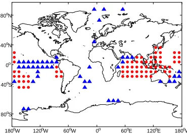
Climate networks were constructed using our proposed network construction methodology with OND rainfall variability in the GHA as the response variable of interest (see Section 2.5). To capture time-lagged relationships, which are often present in climate data, five (5) climate networks were constructed, one for each month, starting four (4) months before the season (June) until the first month of the season (October). It is worth noting that when constructing a climate network for the month of May, no spatial points were selected as potentially associated with the response variable, suggesting that this month may be too early before the season to yield significant climate indices.

Each climate network was constructed using information from four (4) related stations in the North Eastern Highlands of Tanzania. Since these stations are located in the same climatological region and exhibit highly correlated rainfall patterns, they are expected to be associated with the same global climate patterns1. Hence, the use of the consensus set allows us to filter out spatial points with potentially spurious associations with the response variable. For example, the spatial points in the Arctic and the Antarctic in Figure 2.3–two regions with no known association with rainfall variability in the GHA–are filtered out using the consensus set.

180o_W ₁₂₀o_W ₆₀o_W ₀o ₆₀o_E ₁₂₀o_E ₁₈₀o_W

80oS 40o_S

0o

40oN 80o_N

Figure 2.3: Spatial points selected in the month of October to construct the climate network. Blue triangles indicate spatial points selected only for individual stations and red circles indicate spatial points in the consensus set.

1

(38)

2.6.4 Climate Indices Discovered

Communities associated with OND rainfall variability in the GHA were identified in the climate networks constructed using the multi-objective algorithms for response-guided community de-tection based on the Louvain method and simulated annealing described in Section 2.3. We set the value of the weighting parameterαto the multiple of 0.05 in the interval [0.75,1] that yields the set of communities with the highest average association with the response variable over the training set. Lower values ofαwere not considered to ensure that the network partition also has a high modularity value. As explained in Section 2.4, a climate index was constructed for each community identified by computing the spatial average over the community of its representative climate variable (see Figure 2.4).

We compare our climate indices with those discovered using a baseline methodology and a state-of-the-art methodology for climate index discovery [57]. For the baseline methodology, communities were identified in multivariate climate networks (i.e., one network was constructed for all covariates via a combined probability test as described in Section 2.5) using the original Louvain method [7] and the original simulated annealing algorithm for community detection [22]. For the state of the art [57], communities were identified in univariate climate networks (i.e., one network was constructed for each covariate) using Walktrap, a single-objective com-munity detection algorithm that identifies communities by optimizing a distance metric based on random walks [46]. In both cases, the community detection and the network construction processes were performed without taking into account the response variable of interest.

180o_W ₁₂₀o_W ₆₀o_W ₀o ₆₀o_E ₁₂₀o_E ₁₈₀o_W

80o_S

40oS 0o 40o_N

80oN

180o_W ₁₂₀o_W ₆₀o_W ₀o ₆₀o_E ₁₂₀o_E ₁₈₀o_W

80o_S

40oS 0o 40o_N

80oN

(39)

Table 2.1 summarizes the properties of the climate networks constructed and the climate in-dices discovered using each methodology. Given that our response-guided community detection algorithms do not exclusively optimize the “goodness” of the network partitions, our climate networks exhibit a lower modularity than those constructed using single-objective methodolo-gies (0.34 vs. 0.74, 0.75, and 0.59). However, our communities have a higher internal density (0.62 vs. 0.29, 0.28, and 0.47) and a lower internal variability (0.63 and 0.62 vs. 0.77, 0.78, and 0.74), indicating a well-defined structure.

We also observe that, unlike most of the climate indices discovered using the baseline and the state of the art, the majority of our climate indices (66.67%) have a statistically significant linear correlation (p <0.01) with the response variable of interest over the training set. Moreover, our proposed methodology performs significantly (p <0.05) better than the baseline and the state of the art across all stations in terms of the average linear correlation between the climate indices and the response variable of interest over the training set and the test set (see Table 2.2). This shows that, as expected, our proposed methodology is able to discover climate indices more strongly associated with the response variable of interest than those discovered with methodologies that make use of single-objective community detection algorithms.

Table 2.1: Properties of networks constructed and climate indices discovered for OND rain-fall variability in the GHA, using the proposed, baseline, and state-of-the-art (SOTA) [57] methodologies with the Louvain method (LM), simulated annealing (SA) and Walktrap as the community detection algorithms: number of networks (Num Nets), average number of vertices and edges per network (Avg Vtxs, Avg Edges), average modularity (Avg Mod), number of indices (Num Idxs), average number of vertices, standard deviation, and internal density per index (Avg Vtxs, Avg Std, Avg Dens), and percentage of indices with a statistically significant (p < 0.01) linear correlation with the response variable of interest (% Idxs). Best values are highlighted in bold.

Method Algorithm

Networks Indices Significant

Indices

Num Avg Avg Avg Num Avg Avg Avg Num %

Nets Vtxs Edges Mod Idxs Vtxs Std Dens Idxs Idxs

Proposed Adapted LM 5 40.80 169.20 0.34 18 11.33 0.63 0.62 12 66.67 Adapted SA 5 40.80 169.20 0.34 18 11.33 0.62 0.62 12 66.67

(40)

Table 2.2: Average linear correlation with OND rainfall at each station and at the GHA region, over the training set and the test set, of climate indices discovered for OND rainfall variabil-ity in the GHA using the proposed, baseline, and state-of-the-art (SOTA) [57] methodologies with the Louvain method (LM), simulated annealing (SA) and Walktrap as the community detection algorithms. Check marks (X) indicate that our proposed methodology performs sig-nificantly better according to a two-way ANOVA with a significance level of 0.05. Best values are highlighted in bold.

Station

Proposed Baseline SOTA

Adapted LM Adapted SA Original LM Original SA Walktrap

Train Test Train Test Train Test Train Test Train Test

Arusha 0.4436 0.2999 0.4431 0.2848 0.2496 0.2495 0.2489 0.2639 0.1481 0.2261 Kilimanjaro 0.4103 0.3752 0.4300 0.3583 0.2586 0.2437 0.2629 0.2525 0.1567 0.2230 Moshi 0.3629 0.2980 0.3764 0.2791 0.2404 0.2552 0.2317 0.2501 0.1393 0.2481 Same 0.4292 0.3403 0.4341 0.3119 0.2574 0.2111 0.2572 0.2429 0.1589 0.2148 GHA 0.4502 0.3478 0.4614 0.3272 0.2763 0.2356 0.2749 0.2497 0.1558 0.2219

Two-way ANOVA (α= 0.05) _X _X _X _X _X _X

2.6.5 Seasonal Rainfall Prediction

We validate the climate indices discovered using our proposed methodology by assessing their predictive power for OND rainfall in the GHA. To this end, we trained linear regression models to predict rainfall at each station and average rainfall at the region using our climate indices as predictors. As specified in Section 2.6.1, data from 1960 to 1997 was used for training and data from 1998 to 2011 was used for testing. For comparison purposes, linear regression models were also built using the climate indices discovered with the baseline and state-of-the-art [57] methodologies introduced in Section 2.6.4.

In order to avoid overfitting, given the small sample size of the data sets, only the top six (6) climate indices with the highest average correlation with OND rainfall in the GHA over the training set were used to build the models. This number of predictors was selected because it yielded relatively stable performance over the training set across all methodologies (see Figure 2.5). Furthermore, to evaluate the ability of the models to make predictions before the start of the OND rainfall season, all experiments were performed using data up to the month of August (one-month lead time). Climate indices discovered for the months of September and October were reconstructed using August data.

(41)

than those built using climate indices discovered with methodologies that make use of single-objective community detection algorithms (see Figure 2.6). This suggests that climate indices more strongly associated with the response variable of interest, such as the ones discovered using our proposed methodology, have greater predictive power.

1 2 3 4 5 6 7 8

0.35 0.45 0.55 0.65

Training Correlation

Number of Predictors

Proposed (LM) Proposed (SA) Baseline (LM) Baseline (SA) SOTA

Figure 2.5: Average linear correlation between true and predicted rainfall for predictions of OND rainfall at each station in the GHA region over the training set using the proposed, base-line, and state-of-the-art (SOTA) [57] methodologies with the Louvain method (LM), simulated annealing (SA) and Walktrap as the community detection algorithms vs. the number of pre-dictors used to build the regression models. The dashed line indicates the number of prepre-dictors selected for further analysis.

Table 2.3: Linear correlation between true and predicted rainfall (Corr) and RMSE scores for predictions of OND rainfall at each station and at the GHA region from 1998 to 2011 obtained using the proposed, baseline, and state-of-the-art (SOTA) [57] methodologies with the Louvain method (LM), simulated annealing (SA) and Walktrap as the community detection algorithms. Check marks (X) indicate that our proposed methodology performs significantly better ac-cording to a two-way ANOVA with a significance level of 0.05. Best values are highlighted in bold.

Station

Proposed Baseline SOTA

Adapted LM Adapted SA Original LM Original SA Walktrap

Corr RMSE Corr RMSE Corr RMSE Corr RMSE Corr RMSE

Arusha 0.7143 0.5017 0.5869 0.5215 0.2462 0.5023 0.3432 0.6853 0.2034 0.5779 Kilimanjaro 0.7629 0.5034 0.6736 0.5619 0.1844 1.0432 0.2053 0.7477 0.2940 0.7874 Moshi 0.6561 0.4719 0.6564 0.4664 -0.0319 0.5937 0.1059 0.7055 0.3088 0.6231 Same 0.7237 0.4779 0.6896 0.4749 0.1470 0.6796 0.1806 0.6929 0.2575 0.7121 GHA 0.7722 0.4133 0.7425 0.4007 0.1501 0.6316 0.2135 0.6390 0.2665 0.6053

(42)

0.71 0.59 0.25 0.34 0.20 0.76 0.67 0.18 0.21 0.29 0.66 0.66 0.030.11 0.31 0.72 0.69 0.15 0.18 0.26

Arusha Kilimanjaro Moshi Same

Stations 0

0.5 1

Correlation

Proposed (Adapted LM) Proposed (Adapted SA) Baseline (Adapted LM) Baseline (Adapted SA) SOTA

0.50 0.52 0.50 0.69

0.58

0.50 0.56 1.04

0.75 0.79

0.47 0.470.59 0.71

0.62

0.48 0.47

0.68 0.69 0.71

Arusha Kilimanjaro Moshi Same

Stations 0 0.5 1 1.5 RMSE

Proposed (Adapted LM) Proposed (Adapted SA) Baseline (Adapted LM) Baseline (Adapted SA) SOTA

Figure 2.6: Linear correlation between true and predicted rainfall and RMSE scores for predic-tions of OND rainfall at each station in the GHA region from 1998 to 2011 obtained using the proposed, baseline, and state-of-the-art (SOTA) [57] methodologies with the Louvain method (LM), simulated annealing (SA) and Walktrap as the community detection algorithms

We further assess the predictive power of our climate indices by comparing our predictions with the official forecasts of the OND rainfall season issued by the TMA every year on Septem-ber. To this end, the rainfall season for each year was categorized according to the guidelines of the TMA asbelow normal,normal, or above normal (rainfall below 75%, between 75% and 125%, or above 125% of long-term averages, respectively). Long-term averages were computed using the training set. Decision trees to classify the OND rainfall season at each station were trained using data up to the month of August and considering only the top six (6) climate indices discovered using our proposed methodology as predictors. The decision trees were built using the Gini index as the split criterion and were pruned to avoid overfitting.