On the Applications of Bluetooth Probe Data for Freeway Systems.

(1)

WAGNER, JOHN ANDREW. On the Applications of Bluetooth Probe Data for Freeway Systems. (Under the direction of Dr. Billy Williams.)

This thesis examines the viability and applicability of long-term performance studies of greater than 2 months for freeway segments using data from roadside Bluetooth sensors (henceforth known as “Bluetooth probe data”). It also aims to compare observations from these Bluetooth sensors to contemporary observations from INRIX to assess accuracy as well as fundamental advantages and disadvantages of both probe data types.

To accomplish this, three study sites in North Carolina were identified, all 12 to 15 miles in length: Interstate 540 in Raleigh, Interstate 95 in Lumberton, and Interstate 40 in Asheville. Using a set of 4 commercial Bluetooth monitoring devices (BlueMAC), long-term bi-directional studies of several months were conducted at each site.

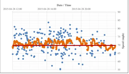
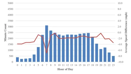
The collected Bluetooth probe data successfully captured point-to-point device observations from which valuable information about the roadway performance was developed. Average Bluetooth observations varied between 300 and 1,600 per day, depending on study site and direction. As expected, travel times collected via Bluetooth provided insight into variation in driver behavior, particularly during free flow conditions. Sampling rates of 5.5%-7.5% were observed along the I-540 Raleigh facility, where volume data was available. Bluetooth observations matched well overall with travel times stitched from INRIX 1-minute data with average speed differences less than 5mph, but some systematic differences were identified; for example, travel times developed from INRIX data lagged behind Bluetooth observations in identifying freeway breakdown conditions by an average of approximately 12 to 15 minutes. Bluetooth probe data also showed speeds averaging about 3-4mph lower than INRIX at the peaks of events. Difficulties with INRIX speed processing were also experienced with up to 11% data loss due to gaps in the 1-minute readings.

(2)

individual drivers both during peaks and throughout the day.

Those individual devices were in turn used to develop travel time distributions, which were then compared to overall Bluetooth travel time distributions across all observed devices both at the 24-hour level and at peak. Not only did the individual device distributions provide valuable contextual information, they also showed distinct patterns at the 24-hour level and the extent of reliability experiences during the peak. During the peak hour, it was also clear that the individual device distributions matched more closely with the overall Bluetooth distribution than with the overall INRIX-derived distribution.

(3)

by

John Andrew Wagner

A thesis submitted to the Graduate Faculty of North Carolina State University

in partial fulfillment of the requirements for the Degree of

Master of Science Civil Engineering

Raleigh, North Carolina 2016

APPROVED BY:

_____________________________ ____________________________ Dr. Nagui Rouphail Dr. George List

___________________________ Dr. Billy Williams

(4)

DEDICATION

Firstly, great thanks go to Dr. Billy Williams, my academic advisor of many years and constant source of advice and encouragement. I would also like to recognize Dr. Nagui Rouphail, director of NC State’s Institute for Transportation Research and Education, as well as Dr. George List, a prominent professor and travel time reliability researcher, for their guidance.

This work was also greatly assisted by many individuals at the North Carolina Department of Transportation, who authorized the data collection used for this project and provided crucial assistance in terms of safety. Particular thanks go to Thomas Elmore, Chuck Miller, and Jason Willis for their consistent support.

I am greatly thankful for the support of the National Transportation Center at the University of Maryland throughout my graduate career. That support has enabled me to more easily pursue my degree, and the research opportunities involved have complimented my graduate studies well.

Additional thanks go to the Federal Highway Administration’s Universities and Grants Programs Office and their facilitation of the Dwight David Eisenhower Graduate Fellowship Program, which I am honored to have taken part in.

(5)

BIOGRAPHY

(6)

TABLE OF CONTENTS

List of Tables ... vii

List of Figures ... ix

Chapter 1. Introduction ...1

1.1 Project Motivation ...1

1.2 Problem Statement, Scope, and Objectives ...3

1.3 Literature Review...4

1.3.1 Bluetooth Studies ...4

1.3.2 INRIX Studies ...8

1.3.3 Bluetooth-INRIX Comparison Studies ...9

1.3.4 Travel Time Reliability ...10

1.4 Thesis Outline ...12

Chapter 2. Data Description and Study Locations ...13

2.1 Study Site Descriptions, Visualizations, and Bluetooth Equipment Setup ...13

2.2 End-to-End Bluetooth Observational Statistics ...18

2.2.1 Site 1 - Raleigh...19

2.2.2 Site 2 – Lumberton...23

2.2.3 Site 3 – Asheville ...27

2.3 Individual Bluetooth Sensor Statistics ...31

2.3.1 Site 1 – Raleigh ...31

2.3.2 Site 2 – Lumberton...32

(7)

2.4 INRIX Data Statistics ...33

Chapter 3. Analysis Process Details and Description ...34

3.1 Raw Data Processing ...34

3.1.1 Bluetooth Probe Installations ...34

3.1.2 INRIX ...37

3.2 Travel Time Comparison Analysis ...38

3.3 Individual Bluetooth Sensor Analysis ...40

3.4 Travel Time Reliability Performance Measure Analysis ...40

3.5 Additional Special Studies ...41

3.5.1 Individual Segment Analysis for Site 1 ...41

3.5.2 Weigh Station Analysis for Sites 2 and 3 ...42

3.5.3 Reliability for Site 1 / Individual Device Reports ...42

Chapter 4. Study Results ...43

4.1 Travel Time and Source Comparison Analysis ...43

4.1.1 Bluetooth Travel Time Trends ...43

4.1.2 INRIX Travel Time Trends ...49

4.1.3 Source Comparison Results ...51

4.2 Individual Bluetooth Sensor Trends and Results ...62

4.2.1 Overall Trends from Hit and Device Counts ...62

4.2.2 Sampling Rate Analyses ...63

4.3 Travel Time Reliability Applicability Analysis ...67

(8)

4.4.1 Individual Segment Analysis for Site 1 ...69

4.4.2 Weigh Station Analysis for Sites 2 and 3 ...73

4.4.3 Reliability for Site 1 / Individual Device Reports ...78

Chapter 5. Discussion of Findings, Observed Trends, and Future Recommendations...88

5.1 Long-Term Bluetooth Study Viability ...88

5.2 Bluetooth-INRIX Comparisons and Resulting Trends ...89

5.3 Reliability Role for Bluetooth Probe Data ...90

5.4 Recommendations for Future Study ...91

References ...94

(9)

LIST OF TABLES

Table 2-1 Study Site Locations and Durations ... 13

Table 2-2 Site 1 Bluetooth Observation Statistics - Eastbound ... 19

Table 2-3 Site 1 Bluetooth Observation Statistics - Westbound... 20

Table 2-4 Site 2 Bluetooth Observation Statistics - Northbound ... 23

Table 2-5 Site 2 Bluetooth Observation Statistics - Southbound ... 24

Table 2-6 Site 3 Bluetooth Observation Statistics - Eastbound ... 27

Table 2-7 Site 3 Bluetooth Observation Statistics - Westbound... 28

Table 2-8 Site 1 Bluetooth Station Detection Statistics ... 31

Table 2-11 INRIX Data Quality Statistics – All Routes ... 33

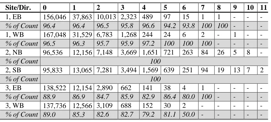
Table 4-1 Study Minutes by Bluetooth Observation Count... 51

Table 4-2 INRIX-Available Study Minutes by Bluetooth Observation Count... 52

Table 4-3 Average Bluetooth Observations Per Minute ... 52

Table 4-4 Bluetooth-INRIX Comparison Measures by INRIX Speed Bin, Site 1 ... 53

Table 4-7 Site 1 Average Bluetooth Station Sampling Rate Estimates ... 66

Table 4-8 Sites 2 and 3 Average Bluetooth Station Sampling Rate Estimates ... 66

(10)

Table 4-10 AM Peak Reliability Measures, Selected Sites and Directions ... 67

Table 4-11 PM Peak Reliability Measures, Selected Sites and Directions... 68

Table 4-12 Site 1 Segmented Bluetooth Observation Counts, Eastbound... 69

Table 4-13 Site 1 Segmented Bluetooth Observation Counts, Westbound ... 69

Table 4-14 24-Hour Monthly Reliability Measures, Site 1 Both Directions ... 79

Table 4-15 AM Peak Monthly Reliability Measures, Site 1 Westbound ... 79

(11)

LIST OF FIGURES

Figure 2-1 Study Site Locations Within North Carolina ... 14

Figure 2-2 Example Bluetooth Sensor Installation ... 16

Figure 2-3 Site 1 (I-540, Raleigh) Bluetooth Sensor Locations ... 17

Figure 2-4 Site 2 (I-95, Lumberton) Bluetooth Sensor Locations ... 17

Figure 2-5 Site 3 (I-40, Asheville) Bluetooth Sensor Locations ... 18

Figure 2-6 Site 1 Eastbound Bluetooth Observations - Weekday ... 21

Figure 2-7 Site 1 Eastbound Bluetooth Observations - Weekend ... 21

Figure 2-8 Site 1 Westbound Bluetooth Observations – Weekday ... 22

Figure 2-9 Site 1 Westbound Bluetooth Observations – Weekend ... 22

Figure 2-10 Site 2 Northbound Bluetooth Observations – Weekday ... 25

Figure 2-11 Site 2 Northbound Bluetooth Observations – Weekend ... 25

Figure 2-12 Site 2 Southbound Bluetooth Observations – Weekday ... 26

Figure 2-13 Site 2 Southbound Bluetooth Observations – Weekend ... 26

Figure 2-14 Site 3 Eastbound Bluetooth Observations – Weekday ... 29

Figure 2-15 Site 3 Eastbound Bluetooth Observations – Weekend ... 29

Figure 2-16 Site 3 Westbound Bluetooth Observations – Weekday ... 30

Figure 2-17 Site 3 Westbound Bluetooth Observations – Weekend ... 30

Figure 4-1 Example Variation Seen Among Free Flowing Bluetooth Observations ... 43

Figure 4-2 Variation Contrast During Congestion Events ... 44

(12)

Figure 4-4 Bluetooth Variation Example 2: Site 1 EB 2015-04-01... 45

Figure 4-7 Bluetooth Variation Example 5: Site 1 WB 2015-03-02 ... 47

Figure 4-11 INRIX Versus Bluetooth Variation During Free Flowing Conditions ... 50

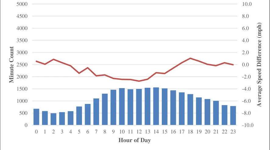
Figure 4-12 Site 1 Eastbound Hourly Count and Average Speed Difference Plot ... 55

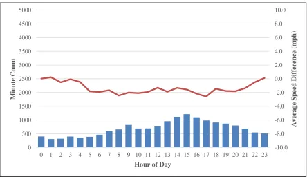
Figure 4-13 Site 1 Westbound Hourly Count and Average Speed Difference Plot ... 55

Figure 4-14 Site 2 Northbound Hourly Count and Average Speed Difference Plot ... 56

Figure 4-15 Site 2 Southbound Hourly Count and Average Speed Difference Plot ... 56

Figure 4-16 Site 3 Eastbound Hourly Count and Average Speed Difference Plot ... 57

Figure 4-17 Site 3 Westbound Hourly Count and Average Speed Difference Plot ... 57

Figure 4-18 Congestion Comparison Example 1: Site 1 Eastbound, 2015-03-19 ... 59

Figure 4-19 Congestion Comparison Example 2: Site 1 Westbound, 2015-04-28 ... 60

Figure 4-20 Congestion Comparison Example 3: Site 1 Westbound, 2015-02-24 ... 61

Figure 4-21 Site 1 Hourly Sampling Rate Histogram ... 63

Figure 4-22 NCSU1 Hourly Average Sampling Rates ... 64

(13)

Figure 4-26 Site 1 Segment-Developed Travel Time Test Plot, EB 2015-04-16 ... 70

Figure 4-27 Site 1 Segment-Developed Congestion Event Plot, EB 2015-04-16 ... 71

Figure 4-28 Site 1 Eastbound Observed and Synthesized Travel Time Distributions ... 72

Figure 4-29 Site 2 SB Weigh Station Segment Travel Time Plot, 2015-08-19 ... 74

Figure 4-30 Site 2 NB Weigh Station Segment Travel Time Plot, 2015-07-29 ... 75

Figure 4-31 Site 2 NB Weigh Station Segment Travel Time Plot, 2015-07-23 ... 76

Figure 4-32 Site 3 EB Weigh Station Segment Travel Time Plot, 2015-11-18 ... 77

Figure 4-33 Site 2 NB End-to-End Daily Plot, 2015-07-23 ... 78

Figure 4-34 Site 1 Eastbound 24-Hour Individual Frequency Histogram ... 81

Figure 4-35 Site 1 Westbound 24-Hour Individual Frequency Histogram ... 81

Figure 4-36 Site 1 Eastbound PM Peak Individual Frequency Histogram ... 82

Figure 4-37 Site 1 Westbound AM Peak Individual Frequency Histogram ... 82

Figure 4-38 Site 1 EB 24-Hour Overall and Device Travel Time Distributions ... 84

Figure 4-39 Site 1 EB PM Peak Overall and Device Travel Time Distributions ... 85

(14)

CHAPTER 1.INTRODUCTION

1.1Project Motivation

As Internet-connected devices like smartphones become more ubiquitous, it is paramount to utilize new communications capabilities to build a more vibrant freeway performance data structure. Bluetooth-enabled devices are already plentiful on the roadway, and their short range can prove advantageous for freeway performance analysis. This research seeks to improve the viability of the application of Bluetooth vehicle data collection systems for freeways in order to expand their role in the fields of freeway operations monitoring and intelligent transportation systems. To accomplish this, it is necessary to achieve a deeper understanding of their effectiveness and develop better practices for their use.

The popularity of probe data has increased significantly in recent years for evaluating the performance of freeways and major arterials, both by state agencies and private firms. The role of probe data in freeway analysis is critical due to its cost-effectiveness and flexibility. Moreover, the process of retrieving probe data is non-intrusive to the traffic stream by definition. As mobile devices and wireless connectivity proliferate among the driving public, collection of probe data from freeway facilities becomes appreciably easier. Bearing this emergence in mind, there are technical and institutional issues that must be examined for all types of probe data.

(15)

While there are many other sources and types of probe data, one prevailing source (and a source of probe data for the North Carolina Department of Transportation) is INRIX, which uses location data from a variety of sources, including mobile phones and GPS-equipped fleet vehicles (e.g. freight trucks, delivery vans) to develop speed profiles on freeways and major arterials. Using “traffic message channels,” or TMCs, to discretize long freeway facilities to manageable analysis lengths, INRIX provides speed data down to a 1-minute resolution. By using the INRIX-defined TMC segment lengths, these speeds can be “stitched” together to calculate synthetic travel times based on the INRIX probe data speeds. The viability of this synthetic process needs to be assessed.

Additionally, concurrent Bluetooth observations provide a real-world benchmark for travel time and facility performance due to their nature as point-to-point observations. Instead of relying on average speeds or other measures developed from aggregated means, Bluetooth probe data allow for more rigorous evaluation of freeways by providing a more defensible data framework.

One primary field of interest for the use of these sources of freeway probe data is that of travel time reliability. Travel time reliability attempts to quantify and classify the long-term performance of a particular roadway facility (typically freeways and arterials), usually by examining a target time-of-day analysis period. While there are many varying definitions and measures of effectiveness under the umbrella of “travel time reliability,” all require a stable and accurate source of travel time data. Both Bluetooth probe data and INRIX probe data fulfill the needs for performance measure calculation in this context of travel time reliability.

(16)

1.2Problem Statement, Scope, and Objectives

Using Bluetooth observations from the field and concurrent INRIX space mean speed data, travel times from selected study sites were developed along with their respective distributions. This research examines those travel times and distributions to determine the effectiveness of long-term freeway studies using Bluetooth probe data and to comment on current technical challenges. In addition, this thesis assesses the applicability of Bluetooth travel time distributions for use in developing travel time reliability performance measures.

This research endeavors to examine probe data studies entirely in the standard freeway context; arterial facilities and facility types like managed freeway facilities (e.g. tollways) are not considered in this research.

The research questions and subsequent objectives are threefold: first, are long-term Bluetooth probe data studies viable for assessing the variable freeway performance on their respective freeway facilities; second, do observed travel times from these Bluetooth probe data studies match well with travel times developed from INRIX probe data; finally, are Bluetooth travel times sufficient in providing a basis to develop travel time reliability performance measures?

To address the question of long-term study viability, freeway studies were performed on diverse sites within the state of North Carolina. Data quality – primarily in terms of total detections and capture percentage – was examined and commented upon.

With respect to the Bluetooth-INRIX comparisons, speed differences were computed on an hourly basis at each site in each direction; aggregation based on speed ranges was also performed. The evaluation of a “stitching” algorithm to generate travel times from INRIX 1-minute space mean speed data was also included in answering this research question.

(17)

ability to identify individual devices and develop device-specific reliability metrics was also assessed in a special additional study.

The initial hypothesis for this project is that Bluetooth probe data will provide a sufficient basis on which to evaluate freeway performance, providing a number of benefits when compared to other methods and data sources. It is also expected that this research will show that Bluetooth probe data will match well with results generated from INRIX space mean speed data.

The end goal of this research is to assess the hypotheses above by evaluating the benefits and effectiveness of long-term (defined here as greater than two months) freeway Bluetooth travel time studies using the study sites detailed in Chapter 2 and the methodology presented in Chapter 3.

1.3Literature Review

In order to establish a baseline of knowledge from related studies and research involving probe data studies (Bluetooth and INRIX alike) and the developing field of travel time reliability, a literature review was performed.

The literature review is categorized into four sections: past studies concerning Bluetooth technology for travel time sensing from the roadway, past studies concerning INRIX probe data for sensing roadway speeds and travel times, past studies comparing Bluetooth and INRIX data (along with other sources, in some cases), and literature discussing the major elements of travel time reliability. The sections below present the relevant points from that literature in that order.

1.3.1Bluetooth Studies

(18)

a series of sensors to collect MAC addresses and associated timestamps and then matching those detections to calculate travel times based on the difference in the timestamps. Most (and nearly all) studies using Bluetooth sensors along the roadway to assess travel times – at least those noted in the available literature – operated solely or primarily within the realm of urban arterials. This research seeks to provide a freeway-only perspective to address this scarcity of freeway Bluetooth studies.

Puckett and Vickich (1) performed a successful deployment of Bluetooth travel time sensing equipment in the city of Houston in 2009 with the goal of device and data processing system development. In an initial deployment, many barriers proved problematic in terms of device development, including temperature and device compatibility. Using antennas with a range of approximately 300 feet, the main installations occurred at arterial intersections. Puckett and Vickich determined that an optimal height for placing the sensors they had developed was at approximately windshield level (~4-5’). Further studies recapped in their report include a small grid deployment of sensors along two parallel arterials. The concept of filtering out travel times irrelevant to the performance of the facility (“outliers”) was noted as particularly difficult in these early tests. The mean and percentage-departure system used in their field applications was described as having intermittent challenges, particularly as actual facility performance deteriorated. While the main appeared to be technical in nature, Puckett and Vickich indeed showed that Bluetooth travel time sensing was possible and viable, at least for short-to-mid-term (~1-2 weeks) arterial studies.

(19)

single-device-per-vehicle assumption. Cost effectiveness of Bluetooth was mentioned as a primary advantage, along with the non-invasive probe nature of the data. Not only were the Bluetooth probe data able to assess travel times along the alternative routes, but they also proved effective in quantifying the distribution of vehicles among the routes.

Kothuri et al. (3) coupled Bluetooth-sensed travel time data with automatic vehicle location (AVL) data from buses during a 3-mile, one-week arterial study in Portland, Oregon in 2010. Using Bluetooth readers and associated travel times, Kothuri et al. sought to examine the possibility that AVL data accurately represented arterial travel times. In the Bluetooth data collection process, four devices were deployed and data was written to mini-computers housed at each installation site. For processing, it was noted that any MAC address-based data collection (like Bluetooth) could not distinguish between two critical sets of characteristics: continuous trips versus discontinuous trips and single-mode trips versus multimodal trips. This limitation necessitated the use of an outlier screening process, for which Kothuri et al. employed a moving standard deviation and mean-based approach. Both the “first-first” and “last-last” methods of MAC address matching were considered (more information on matching options is provided in 3.1.1). Intriguingly, the capture rate for this study was noted as 5-11%, higher than other studies in the recent literature. The AVL data was found to be consistently positively biased when compared to the Bluetooth data (meaning they indicated longer travel times and lower average speeds than Bluetooth), attributed primarily to the periodic stops of the buses.

(20)

years. Mean Percentage Error (MPE), Mean Absolute Percentage Error (MAPE), and Root Mean Squared Error (RMSE) were used as the evaluation criteria. While Bluetooth was found to be an acceptable method for assessing travel time, using the minimum and median travel time observations for reporting purposes was noted as more effective based on the evaluation criteria than the average or maximum values.

Young (5) evaluated Bluetooth travel time technology on a more long-term, permanent reporting basis than the other studies presented here. Six sensor units were deployed for an arterial test study covering most of 2011 (specific length not provided) and evaluated against data gathered from an automatic traffic recorder (ATR). This comparison was found to have promising results in terms of accuracy and reliability of the data. Moreover, further comparison of the Bluetooth test data to toll tag travel time data determined the Bluetooth sensors to have sufficient sampling capabilities to fully characterize the traffic stream in terms of both overall average performance and variation (presumably in the form of standard deviation). Young also commented on sensor installation height; in the performed tests, a sensor height of approximately 10’ was observed to capture about twice the number of devices as a ground-level installation.

(21)

assumptions made in a variety of freeway operations models.

Park and Haghani (7) presented a comparison of various Bluetooth sensor location optimization frameworks: deterministic, stochastic, and dynamic. Such frameworks were commented to be useful for future deployments targeting optimized location and relocation of Bluetooth sensor devices. While much of this work was not directly applicable to the research presented here, Bluetooth probe data were noted as preferable to single-point detection equipment (e.g. inductive loops) because of their nature as point-to-point, representing real-world trips instead of speed estimates attached to a single location.

1.3.2INRIX Studies

INRIX probe data is a popular tool for agencies both public and private for speed assessments because of its wide reach and non-invasive nature as probe data. INRIX uses a variety of data sources in its synthesis process leading to output speed data, including GPS, cellular networks, road sensors, and traffic cameras (8). INRIX data is also used extensively for research purposes in a variety of contexts typically involving major arterials or freeway facilities. Bearing that in mind, several studies have been performed to evaluate the effectiveness and accuracy of INRIX speed data. Unlike the Bluetooth probe data studies, freeways are the primary facility type studied and discussed in the INRIX-related literature.

(22)

alternative method for establishing a comparison benchmark, presumably due to the point-to-point nature mentioned by Park and Haghani (7).

Sisiopiku and Islam (10) utilized INRIX probe data in a study of travel time reliability along Interstate 65 in Birmingham, Alabama in 2010. The travel time reliability elements of their research are discussed in 1.3.4. The INRIX averaging process was described and particular attention was called to the ability to clearly see incident effects from the provided and analyzed data.

Kim and Coifman (11) performed a direct comparison of INRIX probe data to inductive loop data along Interstate 71 near Columbus, Ohio. Several deficiencies or questionable results concerning the INRIX data were identified and discussed. First, INRIX readings were believed to lag the loop detector speeds by about 6 minutes, particularly during congestion or incidents that brought lower speeds. As Kim and Coifman note, such a lag could cause major operational issues with systems that require real-time performance data to function properly (e.g. ramp meters). Secondly, the lack of minor variation and the tendency of INRIX data to repeat reported speeds for several time intervals is discussed. One possible explanation offered by Kim and Coifman was that the granularity of the data processing was not as fine as the data structure suggested, and that reducing any processing delay might eliminate the latency that was identified. Lastly, the measures of confidence associated with INRIX data did not appear to explain either of the prior issues.

1.3.3Bluetooth-INRIX Comparison Studies

While significantly less common than other studies mentioned in this review, there have been efforts made to compare Bluetooth and INRIX probe travel times. These studies provided a foundation on top of which this research attempts to build.

(23)

Bluetooth data was used as the benchmark for the study, and comparison results were compiled into four bins: 0-30mph, 30-45mph, 45-60mph, and >60mph. Average Absolute Speed Error (ASE) and Speed Error Bias (SEB) were the primary evaluation measures. While it was noted that all contractual data quality standards being studied were met, positive speed bias was present with INRIX probe data at lower speeds and negative bias was present at greater than 60mph.

Alhajri (13) performed another Bluetooth and INRIX probe data comparison study while employing separate ground truth runs with GPS-equipped floating cars. This study, unlike that of Haghani, Hamedi, and Sadabadi, took place on a suburban arterial over nine days in the Maryland/Virginia area. Mean Absolute Error (MAE) and Mean Absolute Percentage Error (MAPE) were the primary evaluation measures, and the same 0-30mph, 30-45mph, 45-60mph, and >60mph bins were used. The overall results suggested that both sources could produce reasonably accurate travel times when compared to the floating car data, but there were distinct strengths; INRIX data proved superior for midday applications and Bluetooth data was more accurate in the PM peak. This study also showed that INRIX was more prone to underestimating speeds, particularly near free flow. Alhajri’s study also performed a matched-pairs t-test that determined that the Bluetooth and INRIX mean travel times were significantly different.

1.3.4Travel Time Reliability

(24)

data) have been identified as critical for producing the distributions of travel times necessary to generate these performance measures.

Travel time reliability’s varied application concerning congestion is important to note; not only do its performance measures address regularly occurring congestion (e.g. what one would see with a commuter-heavy facility), but it also encompasses non-recurring events from weather, incidents, and special events. The literature concerning travel time reliability is becoming increasingly extensive, so only the most relevant background literature is described in this review.

Toppen and Wunderlich (14), in a 2003 report, presented the benefits of accurate reporting of travel time and possible methods of reaching these estimates. While travel time reliability had not yet reached maturity as a field, Toppen and Wunderlich outlined the need for accurate travel time reporting and information dissemination from a user-based perspective in terms of an Advanced Traveler Information System (ATIS). Moreover, value is identified for assessment of both accuracy of travel time and the variability within the traffic stream.

Sisiopiku and Islam (10) focused on travel time reliability in their study along Interstate 65 in Alabama, specifically focusing on calculation of performance measures and comparison of INRIX data to the SHRP2 L03 modeling procedure. The selected reliability performance measures that were calculated and analyzed were 90th/95th percentile travel time, Buffer Time Index (BTI), and Planning Time Index (PTI). Significant effects from incident events were observed throughout the study. The L03 model was found to match quite well with the field data; however, particular errors were identified with the PTI values as they increased. Nevertheless, particular value was found in the reliability study and the L03 modeling potential.

(25)

distributions for calculation of performance measures and the associated performance measures themselves. In addition, formal definitions were offered for time-space study area definitions, drawing from the existing HCM freeway segment definitions. Reliability commentary was developed for both freeway facilities and urban street facilities; the freeway perspectives are of more use in this research. The performance measures (and freeway benchmark values) described by Kittelson and Vandehey will constitute the majority of the characterizing comparison metrics presented in this research.

Schroeder, Rouphail, and Aghdashi (16) laid critical groundwork for the field of travel time reliability by outlining a core methodology for assessing it on freeways, developed from the SHRP L08 findings. A scenario generation process was developed to incorporate a variety of variables impacting traffic stream performance, and by extension, travel time reliability: demand variability (time, day, and month), work zones, incidents, and weather impacts. Emphasizing the need for apples-to-apples comparisons for reliability, they noted that performance measures indexed to free-flow speeds (e.g. TTI, PTI) were preferable to travel time or speed metrics because of the contextual advantages they provide. In a case study and model calibration along Interstate 40 in Raleigh, North Carolina, the viability of their method was successfully demonstrated when compared to travel time distributions developed from INRIX data. Interestingly, INRIX travel times possessed a higher percentage of travel times close to free flow than the model, hinting at the biases discussed in other INRIX-based studies.

1.4Thesis Outline

(26)

CHAPTER 2.DATA DESCRIPTION AND STUDY LOCATIONS

Three study areas from the state of North Carolina were selected to represent different facility trends, prevailing uses, and geographic conditions. Table 2-1 displays these study site locations along with some basic information on each. Analysis for this research was conducted in both directions for each study site facility.

Table 2-1 Study Site Locations and Durations

# Facility Metro Area Length Study Start/End Dates SL Duration

1 I-540 Raleigh, NC 12.7mi 2014-01-09 to 2015-06-10 70mph 5 mo. 2 I-95 Lumberton, NC 14.5mi 2015-06-15 to 2015-09-01 65mph 2.5 mo. 3 I-40 Asheville, NC 13.9mi 2015-10-21 to 2016-02-21 60mph 4 mo.

Tools from the Vehicle Probe Project (vpp.ritis.org) were used to identify interstate candidate sites based on historic levels of congestion and delay. Study sites were selected at the outset of the project to include diverse population density and geographic area type, terrain, and prevailing facility use (e.g. commuter, freight, mixed). The selected study sites listed above and detailed in 2.1 represented what were interpreted to be the most useful locations for observation based on these criteria.

2.1Study Site Descriptions, Visualizations, and Bluetooth Equipment Setup

The three selected study sites are shown in the context of the state of North Carolina in Figure 2-1 on the next page as follows:

 Site 1, I-540 in Raleigh, is shown in red.

 Site 2, I-95 in Lumberton, is shown in blue.

(27)

Figure 2-1 Study Site Locations Within North Carolina

Site 1, a 12.7-mile section of Interstate 540 in the northern area of Raleigh, is primarily a commuter route to and from the Research Triangle Park (RTP), located to the west of the study area between Raleigh and Durham. In addition, this section of I-540 runs adjacent to Raleigh-Durham International Airport (RDU), a major source of trips in this area of Raleigh, at its western end. As such, Site 1 provided a study facility located in a large urban environment that showed consistent, reliable congestion from commuter traffic in weekday peaks. This congestion was at times exacerbated by the presence of incidents and weather events. Limited non-peak congestion events/incidents were also observed.

(28)

area, about 2 miles from the northernmost point. The presence of a weigh station in the study area presented a trio of analytical challenges: first, increased Bluetooth travel times from freight vehicles not necessarily from deteriorating travel conditions; second, the heightened opportunity for discrepancies between Bluetooth and INRIX-derived observations; finally, the possibility of truck queue spillback from the weigh station into the main travel lanes. The weigh station issue is expounded upon in 4.4.2.

Site 3, a 13.9-mile section of Interstate 40 in the southern area of Asheville, represented a mix between local traffic (including commuters) and through traffic (including freight). Asheville, while an urban area, is considerably smaller than Raleigh, offering less commuter traffic leading to less consistent congestion along this study site route. Site 3, like Site 2, contains a weigh station, providing another environment for observing effects from such a facility. Another potential source of delay and complexity for this study site was a work zone on Interstate 26 just south of the study facility; I-26 has a large interchange with I-40 inside of the study site, and that interchange was a primary source of complexity and congestion.

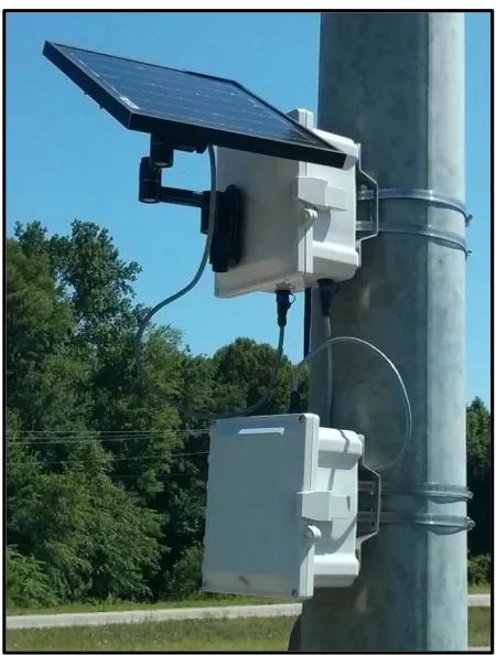
Each study site employed four commercial Bluetooth sensors, with one sensor at each endpoint and two intermittent sensors placed at roughly the one-third and two-third points along the study facilities; Bluetooth sensor spacing ranged between 3 and 6 miles. The Bluetooth sensors used were fifth-generation BlueMAC units, manufactured by Digiwest LLC. Figure 2-2 on the next page provides a representative setup of the sensor equipment from the Site 2 study in Lumberton (NCSU4).

(29)

Figure 2-2 Example Bluetooth Sensor Installation

Figure 2-2 above shows the basic elements of the Bluetooth sensor deployment used at the study sites. The top unit is the main operating structure, housing one 12V 12Ah battery, a GSM mobile radio, the Bluetooth radio and antenna proper, and a solar charging assembly. The solar charging panel is mounted on the front of this top unit and is adjusted in the field for maximum efficiency. The bottom unit is the supplementary battery pack, housing two additional 12V 12Ah batteries. The battery pack and the solar panel are connected to the top unit via umbilicals. Both units are mounted to an existing pole or other available infrastructure using metal brackets and straps as shown. Supplementary battery packs were not used for most of the Site 1 study, but were part of the sensor installations for the studies at Sites 2 and 3.

(30)

Figure 2-3 Site 1 (I-540, Raleigh) Bluetooth Sensor Locations

(31)

Figure 2-5 Site 3 (I-40, Asheville) Bluetooth Sensor Locations

The study sites were set up as close as possible to endpoints of INRIX TMC segments to minimize the need for adjustments when comparing Bluetooth and INRIX-derived travel times. Nevertheless, necessary infrastructure was not available to completely avoid such adjustments, which are detailed in 3.2.

For the duration of each study, all Bluetooth sensors operated in the 20dB (Class 1) mode.

2.2End-to-End Bluetooth Observational Statistics

Each of the three studies produced tens of thousands of observed trips in each direction; while some of these trips were outliers not representative of the traffic stream, the majority of the observations provided useful information. Others, while not outlying values, occurred on holidays or on weekends. In the following tables, Bluetooth observations are broken down into the following totals, based on the start time of the device trip:

 Number of total Bluetooth observations, regardless of outlier flag or observed day

 Number of total observations with federal holidays excluded

 Number of observations on weekdays only (holidays excluded)

 Number of observations on weekends only (holidays excluded)

 Number of non-outlying observations on weekdays only (holidays excluded)

(32)

For details on data processing, including a description of the process for determining outlying trip times, see 3.1.1. Hour-by-hour counts and plots were developed for weekends and weekdays to show the directional trends of each study route.

2.2.1Site 1 - Raleigh

Table 2-2 Site 1 Bluetooth Observation Statistics - Eastbound

Description Count % of Raw Data

Total Raw Trips 75,396 100.00%

Non-Holiday 73,876 97.98%

Weekday Non-Holiday 59,344 78.71% Weekend Non-Holiday 14,532 19.27% Weekday Non-Outliers 56,290 74.66% Weekend Non-Outliers 13,654 18.11%

Total Usable Obs. 69,944 92.77%

Table 2-2 above shows the core statistics for the eastbound direction of the Interstate 540 study area in Raleigh. For reference, the study period included 108 weekdays, 3 of which were holidays (Martin Luther King, Jr. Day, Washington’s Birthday, Memorial Day). The study period also included 44 weekend days, including one major holiday (Easter Sunday) that while not a federal holiday, was excluded from the analysis dataset. Bluetooth observations were unavailable for 9 weekdays and 4 weekend days during this study, leaving 96 non-holiday weekdays and 39 holiday weekend days with Bluetooth observations. Average non-outlier observations per day for the eastbound direction therefore were approximately 586 per weekday and 350 per weekend day.

(33)

Table 2-3 Site 1 Bluetooth Observation Statistics - Westbound

Total Raw Trips 55,966 100.00%

Total Usable Obs. 52,063 93.02%

Average non-outlier Bluetooth observations per day for the westbound direction, as derived from the table, were approximately 478 per weekday and 236 per weekend day.

These tables, while summarizing data from the same facility, appear on the surface to reflect a clear directional difference. As will be discussed later in Chapter 4, the solar charging issues encountered during the Site 1 study created the appearance of a directional imbalance.

(34)

Figure 2-6 Site 1 Eastbound Bluetooth Observations - Weekday

Figure 2-7 Site 1 Eastbound Bluetooth Observations - Weekend

0 1000 2000 3000 4000 5000 6000 7000

0 1 2 3 4 5 6 7 8 9 10 11 12 13 14 15 16 17 18 19 20 21 22 23

T o ta l Scr ee ned O bs er v a tio ns in Study P er io d

Hour of Day

0 200 400 600 800 1000 1200

0 1 2 3 4 5 6 7 8 9 10 11 12 13 14 15 16 17 18 19 20 21 22 23

(35)

Figure 2-8 Site 1 Westbound Bluetooth Observations – Weekday

Figure 2-9 Site 1 Westbound Bluetooth Observations – Weekend

0 500 1000 1500 2000 2500 3000 3500 4000 4500 5000

0 1 2 3 4 5 6 7 8 9 10 11 12 13 14 15 16 17 18 19 20 21 22 23

Hour of Day

0 100 200 300 400 500 600 700

0 1 2 3 4 5 6 7 8 9 10 11 12 13 14 15 16 17 18 19 20 21 22 23

(36)

2.2.2Site 2 – Lumberton

Table 2-4 Site 2 Bluetooth Observation Statistics - Northbound

Total Raw Trips 120,955 100.00%

Non-Holiday 117,530 97.17%

Total Usable Obs. 110,632 91.46%

Table 2-4 above shows the core statistics for the northbound direction of the Interstate 95 study area in Lumberton. The study period included 57 weekdays, one of which was a holiday: Independence Day, observed on July 3rd. It also included 23 weekend days, including July 4th that while not a technically a federal holiday, was excluded from the analysis dataset. Bluetooth observations were unavailable for 9 weekdays and 4 weekend days during this study, leaving 47 non-holiday weekdays and 18 non-holiday weekend days with Bluetooth observations. Average non-outlier observations per day for the northbound direction therefore were approximately 1,635 per weekday and 1,878 per weekend day.

(37)

Table 2-5 Site 2 Bluetooth Observation Statistics - Southbound

Total Raw Trips 107,578 100.00%

Non-Holiday 103,818 96.50%

Total Usable Obs. 98,045 91.14%

Average non-outlier Bluetooth observations per day for the southbound direction, as derived from the table, were approximately 1,463 per weekday and 1,627 per weekend day.

These tables reflect roughly the same trends, while it is not readily apparent why the northbound direction yielded about 12% more trips than the southbound direction. Unlike Site 1, a commuter facility, a higher proportion of weekend trips were observed on Site 2.

(38)

Figure 2-10 Site 2 Northbound Bluetooth Observations – Weekday

Figure 2-11 Site 2 Northbound Bluetooth Observations – Weekend

0 1000 2000 3000 4000 5000 6000

0 1 2 3 4 5 6 7 8 9 10 11 12 13 14 15 16 17 18 19 20 21 22 23

Hour of Day

0 500 1000 1500 2000 2500 3000

0 1 2 3 4 5 6 7 8 9 10 11 12 13 14 15 16 17 18 19 20 21 22 23

(39)

Figure 2-12 Site 2 Southbound Bluetooth Observations – Weekday

Figure 2-13 Site 2 Southbound Bluetooth Observations – Weekend

0 1000 2000 3000 4000 5000 6000

0 1 2 3 4 5 6 7 8 9 10 11 12 13 14 15 16 17 18 19 20 21 22 23

Hour of Day

0 500 1000 1500 2000 2500

0 1 2 3 4 5 6 7 8 9 10 11 12 13 14 15 16 17 18 19 20 21 22 23

(40)

2.2.3Site 3 – Asheville

Table 2-6 Site 3 Bluetooth Observation Statistics - Eastbound

Total Raw Trips 26,144 100.00%

Total Usable Obs. 24,087 92.14%

Table 2-6 above shows the core statistics for the northbound direction of the Interstate 40 study area in Asheville. The study period included 88 weekdays, six of which were holidays: Veterans’ Day, Thanksgiving Day, Christmas Day, New Year’s Day, Martin Luther King, Jr. Day, and Washington’s Birthday. The study period also included 36 weekend days, none of which were holidays. Bluetooth observations were unavailable for 37 weekdays and 18 weekend days during this study, leaving 45 non-holiday weekdays and 18 non-holiday weekend days with Bluetooth observations. Average non-outlier observations per day for the eastbound direction therefore were approximately 409 per weekday and 316 per weekend day.

(41)

Table 2-7 Site 3 Bluetooth Observation Statistics - Westbound

Total Raw Trips 27,523 100.00%

Total Usable Obs. 25,725 93.46%

Average non-outlier Bluetooth observations per day for the westbound direction, as derived from the table, were approximately 463 per weekday and 272 per weekend day.

These statistics show a close to even split between the eastbound and westbound directions, with slightly more (~5%) eastbound observations. It should be noted that there were significant continuity issues encountered with this study site, causing a lower number of overall observations in both directions. On a per-day basis, however, Bluetooth observations were on par with the other study sites.

(42)

Figure 2-14 Site 3 Eastbound Bluetooth Observations – Weekday

Figure 2-15 Site 3 Eastbound Bluetooth Observations – Weekend

0 200 400 600 800 1000 1200 1400

0 1 2 3 4 5 6 7 8 9 10 11 12 13 14 15 16 17 18 19 20 21 22 23

Hour of Day

0 50 100 150 200 250 300 350 400 450

0 1 2 3 4 5 6 7 8 9 10 11 12 13 14 15 16 17 18 19 20 21 22 23

(43)

Figure 2-16 Site 3 Westbound Bluetooth Observations – Weekday

Figure 2-17 Site 3 Westbound Bluetooth Observations – Weekend

0 200 400 600 800 1000 1200 1400 1600 1800

0 1 2 3 4 5 6 7 8 9 10 11 12 13 14 15 16 17 18 19 20 21 22 23

Hour of Day

0 50 100 150 200 250 300 350 400 450

0 1 2 3 4 5 6 7 8 9 10 11 12 13 14 15 16 17 18 19 20 21 22 23

(44)

2.3Individual Bluetooth Sensor Statistics

Each of the 12 Bluetooth sensor installations (4 at each of the 3 study sites) produced a number of Bluetooth device detections, which are described in greater detail in Chapter 3.

These detections (note: not travel time observations) are of interest because they provide insight into the sampling rate and number of “hits” associated per detection. The BlueMAC sensors’ online portal provides this information automatically, with reports generated in 1-hour time intervals. Those 1-hour reports were used to generate the statistics presented below.

In the tables below, “total devices” refers to the unique number of detections of devices, not the total number of unique devices. No days were removed from these statistics, as the performance of the sensor units is not influenced by holidays or special events.

The “average hits per device” statistic is of particular interest because it gives a sense of the quality of opportunity for the Bluetooth sensor to detect a device as it passes by. This measure allows for a better understanding of potential line of sight deficiencies created by local roadway geometry.

2.3.1Site 1 – Raleigh

Table 2-8 Site 1 Bluetooth Station Detection Statistics

Station Total Hits Total Devices Avg Hits/Device

NCSU1* 1,945,718 512,179 3.799

NCSU2* 2,020,518 426,932 4.733

NCSU3 3,928,291 525,888 7.470

NCSU4 2,639,503 522,484 5.052

(45)

Much of the disparity found in the station statistics above can be attributed to the inconsistency of the solar charging at Site 1, though the high hits-to-device ratio found at NCSU3 is of useful interest.

2.3.2Site 2 – Lumberton

NCSU1 1,929,062 321,568 5.999

NCSU2 1,357,821 328,761 4.130

NCSU3 2,466,794 397,982 6.198

NCSU4 1,526,635 378,862 4.030

With fewer gaps in the data, the detections and devices for Site 2 are more consistent than for Site 1, though NCSU3 still showed a higher hit-to-device ratio than the other stations.

2.3.3Site 3 – Asheville

NCSU1* 1,551,538 227,582 6.817

NCSU2 917,179 309,903 2.960

NCSU3 1,824,349 333,544 5.470

NCSU4 1,694,781 309,424 5.477

*NCSU1 was replaced between the studies at Site 2 and Site 3 after water damage following the end of the Site 2 study.

(46)

2.4INRIX Data Statistics

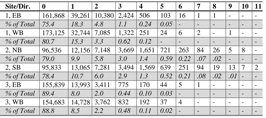
The INRIX data statistics are much simpler in nature. For each site, 1-minute speeds were obtained for each TMC along the route (bi-directionally), meaning there were 1,440 possible speed records for each TMC for each day in the study period and 1,440 possible stitched travel time readings. On occasion, the time between INRIX readings exceeded one minute, leading to fewer than 1,440 readings in one day and causing gaps in the stitched readings; even a one-minute gap in processing can lead to the stitching algorithm missing ten one-minutes or more in creating stitched INRIX travel times. The statistics presented in Table 2-11 on the next page show basic data quality based on gaps in those stitched travel time readings. To better assess INRIX data quality directly compared to the Bluetooth observation dataset, the same holidays in each study period as described in earlier sections were removed for the statistics below.

Table 2-11 INRIX Data Quality Statistics – All Routes

Site/Dir. Records Poss. Actual Total % Gaps

1, EB 213,120 205,408 3.619%

1, WB 213,120 205,465 3.592%

2, NB 112,320 112,320 0.000%

2, SB 112,320 112,320 0.000%

3, EB 174,240 154,413 11.379%

3, WB 174,240 154,283 11.454%

(47)

CHAPTER 3.ANALYSIS PROCESS DETAILS AND DESCRIPTION

Data analysis for this research was conducted in two phases: the processing of the raw data from each source to create travel times for each study and the comparison analysis of those travel times for each study. The first phase of raw data to travel times differs for each data source and will thus be presented separately.

Process details presented in subsequent sections are applicable to all study sites and are for a general case. For travel time data processing, only end-to-end trips (sensor 1 to sensor 4 and vice versa) were considered, as internal Bluetooth segments did not match well with INRIX TMC endpoints in most cases.

3.1Raw Data Processing

3.1.1Bluetooth Probe Installations

For the duration of each study, each Bluetooth sensor unit recorded one line/record of raw data for each detection of a Bluetooth device in its vicinity. This record includes the date and time of the detection, a partial media access control (MAC) address identifying the device, and the received signal strength indication (RSSI). As a device passes by the sensor unit, it is typically detected many times; for a 100-meter Bluetooth detection range, a vehicle traveling at a free-flow speed of 65mph would take about 7 seconds to pass through a sensor’s detection zone. All of the individual detections are written to file as separate records.

There are two main steps in distilling the raw Bluetooth device detections into travel time records: converting the individual Bluetooth detections into single-time records and matching those records based on MAC address.

(48)

information. To convert the BlueMAC raw data into BluStats-friendly format, a Python script was developed. The full code of this Python script is available in the Appendix.

The first step of binding individual detections into single-time records (known within BluStats as the “station” phase) involves only one parameter: the station gapout. Station gapout specifies the amount of time between Bluetooth device detections for a specific device before a single-time record is created and the program “gaps out” to create a new detection for a device. For this research, the default station gapout value was left unchanged at 60 seconds. Theoretically, the station gapout can be adjusted much lower than 60 seconds with little change in results, but the decision was made after brief testing that the default value should be kept for simplicity and convenience in repeated studies.

The second step of deriving the Bluetooth travel times from these device detections is slightly more complex. In BluStats, this step is known as the “segments” phase. For this step, a number of options are presented. The first is the search window, for which a minimum travel time and maximum travel time must be set for each segment. Recall that only the end-to-end travel time segments (i.e. Segment 1-to-4 and Segment 4-to-1) are being considered. Bearing in mind the maximum levels of observed congestion and the length of the study facilities, the minimum time was kept at the default of 0 minutes and the maximum time was increased from the default to a value of 45 minutes. Secondly, the matching algorithm must be specified. At both ends of the study route (upstream and downstream stations), a setting must be defined for what BluStats refers to as the “time tag.” There are nine total algorithm options, made up of three options for this setting for each end:

 First, which is simply the time of the first individual device detection (or the first detection after the gapout time has passed for a particular device)

 Middle, the average time of the First and Last options presented here

(49)

Each of these options was tested for each study, and upon observing the results it was determined that the First-First algorithm (using the First setting at both the upstream and downstream stations) was the most effective for accurately deriving Bluetooth travel times, rather than the default algorithm of Middle-Middle or the alternative of Last-Last. The differences between the methods were admittedly subtle, but the selection of the First-First algorithm originated from three characteristics:

 Algorithms with differing approaches for the beginning and ending stations (e.g. Last-First, Middle-Last) were not preferred due to the adjacent segment analysis to be conducted at Site 1.

 The “Middle” setting averaged two different measurements at each station, meaning that two sources of detection error were present as opposed to one (either the first or last hit)

 First-First allowed for slightly better travel time detection in congestion events where queue accumulation extended upstream of the first station; this is suspected to have happened multiple times at Site 1. The delay in the zone upstream of that first station is considered when using First-First, but not with Last-Last.

(50)

Finally, these matched Bluetooth travel times are written to an output file, one per line, comma delimited, with eight fields: the MAC address, an ID number, the beginning date, the beginning time, the ending date, the ending time, the travel time in minutes, and an “outlier flag” (set to 0 if not an outlier and 1 if an outlier). These travel times were then used for the analysis detailed in 3.2.

3.1.2INRIX

INRIX raw data processing was considerably simpler when compared to that of the Bluetooth sensor stations. Bi-directional data for each route was downloaded from the Vehicle Probe Project (VPP) with a one-minute resolution. In the downloaded data, individual records are given for each TMC segment with the average space mean speed for each minute in the requested dataset. Additionally, a “confidence score” and “c-value” are provided. The “confidence score” is the more important value here, as it provides information concerning the basis of the reported speed in a TMC. The “confidence score” can take three values (13):

 30: The reported speed is wholly based on real-time probe data

 20: The reported speed is based partially on real-time probe data and partially on historical speed data

 10: The reported speed is wholly based on historical speed data

The “c-value” is an additional percentage-based value reporting confidence in those readings with a “confidence score” of 30 – those based entirely on real-time probe data. In general, “confidence scores” of 20 are rare, and values of 10 typically appear in low-demand off-peak hours only.

(51)

This process requires a pre-processing step for the INRIX space mean speed records: using the list of TMCs in one direction, a script using data processing and statistical analysis software program SAS re-formats the raw data (with one line per minute per TMC segment) into a more compact format, providing the date and time in the leftmost column and space mean speed for each TMC segment along one direction of the study route (in travel order) in each subsequent column moving left to right.

Coupling these re-formatted space mean speeds from INRIX with the segment lengths and free flow speeds for the study area, the stitching algorithm calculates travel times for each segment based on the segment lengths and the set of space mean speeds per minute and then adds these together to arrive at the target set of minute-by-minute theoretical travel times.

An important distinction in the INRIX data processing procedures is between the concepts of a “simultaneous” travel time and a truly “stitched” travel time. A simultaneous travel time developed from INRIX data simply involves calculating travel times for each TMC segment based on a single 1-minute interval and adding them together. A stitched travel time is developed using the process described above; this process is significantly more realistic an

The theoretical travel times for each study facility for this research were developed using this process and used for comparison in the process described in 3.2.

3.2Travel Time Comparison Analysis

For comparing the travel times along each study route derived from the raw data from Bluetooth sensors and INRIX speeds, three potential comparison techniques were considered:

 Minute-by-minute averaging, in which Bluetooth results are averaged per minute to match the framework of the INRIX travel time results and compared

 Direct matching of INRIX travel times to Bluetooth results based on start times for Bluetooth-observed trips (non-outliers)

(52)

Based on data coverage (specifically Bluetooth observations), the first option was used for comparison analysis in the context of this section of the research, but that process was not used in the development of travel time distributions needed for the travel time reliability analysis set forth in 3.4; pure Bluetooth travel time distributions were used for that purpose, as they represented real-world trips made between study site endpoints rather than theoretical travel times (as in the case of INRIX).

To adequately compare the performance described by both sets of data, the data needed to be normalized to account for the differences in the study area lengths defined by the Bluetooth sensor locations and the INRIX TMC endpoints. Lengths for each site and direction for Bluetooth and INRIX were measured on Google Earth, and speeds were calculated for each travel time observation. It should be noted that these speeds represent average speeds end-to-end over the entire study area. Travel rates (again, average over the entire study area and direction) were also calculated for each record using these speeds.

To properly compare the screened Bluetooth observations to the stitched INRIX travel times, the VLOOKUP() function in Microsoft Excel was used. The start time for each Bluetooth observation was rounded to the nearest whole minute to create an index minute; for example, 11:25:06 was rounded down to 11:25:00 and 6:47:30 was rounded up to 6:48:00. Mean non-outlier Bluetooth readings were computed per minute when data was available, and further analysis of data quantity was conducted based on number of Bluetooth observations per index minute.

For each minute where data from both Bluetooth and INRIX were available, Average speed difference was calculated between the average Bluetooth observed speed and the stitched INRIX travel speed. It should be noted that these speed differences corresponded to the index minutes for which they were computed; that is to say, they represented the observed speeds for vehicles beginning a trip through the study area at the index minute time.

(53)

involved the aggregated means per minute for both data sources as well as sample size and standard deviation.

3.3Individual Bluetooth Sensor Analysis

Some of the Bluetooth sensor analysis originated in the statistical tables presented in Chapter 2; however, the main focus in this portion of the project was on sampling rate. With the availability of side-fire radar data from HERE.com along Site 1, a more rigorous hour-by-hour examination of sampling rate was conducted. Summary statistics processed by BlueMAC and downloaded from the system’s online portal aggregated unique devices per hour to provide a measure of Bluetooth sensor performance. Using side-fire radar downloaded from HERE.com, volumes for the period of February 2 to February 28, 2015 were aggregated (bi-directionally) at the most adjacent HERE stations to the Bluetooth sensors to most faithfully represent the volumes passing by them. Sampling rate was computed as the ratio (per hour) of unique devices identified by a Bluetooth sensor to the bi-directional volume computed from the adjacent HERE station. Computed sampling rate was then averaged per hour-of-day and plotted on that basis.

For Sites 2 and 3, a similar but less detailed analysis was conducted using AADT counts from NCDOT (18) to approximate long-term sampling rate at each Bluetooth sensor installation. While not as precise, these analyses allowed for a high-level examination of consistency in sampling rate from study site to study site.

3.4Travel Time Reliability Performance Measure Analysis

Using the screened Bluetooth observations from each study site, the following travel time reliability performance measures were developed along with distribution plots for each direction at each study site:

 Planning Time Index (PTI)

 50th_{-percentile Travel Time Index (TTI)}

(54)

 Buffer Time

 Misery Time

Each of these performance measures provides valuable insight into facility performance. Planning Time Index, the ratio of the measured 95th-percentile travel time to the travel time at free flow, presents an assessment of the threshold at which a typical commuter would experience worse conditions approximately once a month (4 weeks, 5 weekdays each) within a given study time-of-day period. Likewise, the 50th-percentile TTI calculates the same ratio for a median trip. Reliability rating (as described above) is a useful high-level performance measure that is calculated in terms of travel time index instead of percentile measurement, allowing for evaluation of more typical operation rather than worst-case scenarios (15).

Buffer time and misery time are more user-based measures. Buffer time measures the additional travel needed to be added to the average travel time to reach an on-time percentage of 95%, while misery time averages the highest 5% of travel times to approximate the average worst-case experience for a user in the study period. Travel time distributions possess more variation at the top of the distribution (where delayed travel times exist), and misery time allows for a rudimentary approximation of conditions in that tail (15).

Commentary resulting from these calculated performance measures was then developed.

3.5Additional Special Studies

Several opportunities for separate special study were identified throughout the data collection, monitoring, and analysis processes. The additional studies’ methodologies are detailed in the sections below.

3.5.1Individual Segment Analysis for Site 1

(55)

comparisons. This analysis mostly involved qualitative conclusions drawn from plots, but a numerical analysis of the number of matches between the devices was also a part of this special study.

3.5.2Weigh Station Analysis for Sites 2 and 3

One of the unique challenges at two of the selected study sites was the presence of a weigh station. Weigh stations provide two sources of instability for travel time as mentioned in the study site descriptions: Bluetooth devices on freight vehicles showing higher travel times after waiting at a weigh station and the freight vehicle queue spillback possibilities that can influence freeway performance upstream of the weigh station. To further examine this challenge, analysis of the Bluetooth matches was performed to estimate percentage of potential weigh station observations and qualitatively comment on more in-depth analysis challenges.

3.5.3Reliability for Site 1 / Individual Device Reports