Nested sliding window protocols with packet fragmentation

Nested Sliding Window Protocols

with Packet Fragmentation

Gerald

W.

Shapiro

and

Harry G.

Perras

Center for Communications and Signal Processing

Electrical and Computer Engineering Department

North

Carolina State University

CCSP TR-89/15

Nested Sliding Window Protocols With Packet Fragmentation'

Gerald W. Shapiro

Department of Management Science

VPI & SU

Blacksburg, VA 24061-0235

Harry G. Perros

Department of Computer Science North Carolina State University

Raleigh, NC 27695-8206

ABSTRACT

A single-hop OSI structured network with multiple layers of sliding window flow control and

packet fragmentation between layers is analyzed. An approximation algorithm is presented

to hierarchically reduce the network to a single queue whose performance characteristics

represent the original network. Network transmission characteristics are restricted to Erlang

distributions. Validation against exact and simulation results showed that the approximation

algorithm has a satisfactory error level.

I. INTRODUCTION

Most modern communication network protocols are designed using a layered structure along

the lines of the OSI model [1]. A common means of implementing the required sequencing,

pactng, congestion control, and data integrity functions of a protocol layer is a sliding window

protocol [1J. Under such a protocol each data packet at a given layer in the sender is given

a number in the range 0 to W-1. W is the window size of this layer. Upon successful receipt

of a data packet, the receiving protocol peer generates an acknowledgment packet for the

sender, indicating the number of the received data packet. Once the acknowledgment is

re-ceived by the sender, the packet number can be re-used to send another packet. If at any time

the sender has W unacknowledged packets outstanding, that sender is blocked and cannot

pass another packet to the layer below it until an acknowledgment for one of the outstanding

1 Supported in part by AIRMICS via the North Carolina State University Center for Communications

packets arrives. There are a number of variants on this basic scheme used in practice, (see

[2]).

Within a given hop, more than one protocol layer may have a sliding window scheme. In such

a situation each protocol layer will have its own window size and packet numbers, and the

sliding window schemes are such that one is imbedded within the other. We refer to this

structure as nested window protocols.

Each layer may have a maximum size data unit it can process, the maximum packet size of

that layer. When a layer at the sending station, say layer l, has a larger maximum packet size

than the layer below it, (layer i - 1), it may be necessary to split the packet from layeri into a

number of smaller packets. This process is referred to as fragmentation of the higher layer

data packet. The peer layer i - 1 at the receiving station must reassemble the fragments

be-fore passing the original data up to the layer i above it.

Of interest to network designers are the throughput and delay performance characteristics of

networks using sliding window protocols. Since the sending layers will periodically be

blocked, the effective transmission capability of the network is less than the raw transmission

rate.

Even simplified models of the sliding window protocol have resisted efforts to date to find

ex-act closed form solutions for the performance measures, (although numerical techniques

in-volvinq the analysis of the underlying Markov chain may be applied to fairly small examples.)

Current analysis depends upon approximation techniques.

Sliding window protocols were analyzed originally (see (3)-[6]) using a closed queueing

net-work with population W. This implies that packets do not enqueue at a blocked sender, but

rather that packets arriving to a blocked sender are "lost". Such models do not accurately

represent the total delay characteristics of packet delivery. Lam (7) presents a general

mod-elling framework which can model a sliding window protocol under this loss assumption.

The models described above deal with only a single layer of sliding window control, and do

not include packet fragmentation. Goto, Takahashi, and Hasegawa [9] and Akyildiz [10]

ana-lyze a model which limits the number of packets allowed at each intermediate station between

the sender and receiver by blocking the downstream neighbor of a full station, in addition to

limiting the number of packets in the end to end connection by the loss assumption. This

comes closer to modelling nested stiding window schemes, but no acknowledgment

mech-anism is modeled, nor is packet fragmentation.

An analysis useful for predicting the maximum throughput of a sliding window controlled link

is presented by Kleinrock and Kermani [11]. In this analysis there is always a packet waiting

for a returning acknowledgment. Fragmentation and nesting are not considered.

Reiser [12] and Thomasian and Bay [13], use a flow-equivalent server technique to model the

sliding window link as a single server queue with state dependent service rate. In this

ap-proach the acknowledgment packets do not explicitly appear in the approximating queue; the

effect of delays due to all sequence numbers in use is accounted for in the delivery service

time of the equivalent server. While these models do not consider fragmentation, they do

explicitly model the delay of packets enqueued at a blocked sender.

Modelling approaches similar to the above are used by Gihr and Kuehn (14l, Varghese, Chou

and Nilsson (15), and Schwartz (16]. In Gihr and Kuehn's analysis the characteristics of the

physical transmission process are obtained from analysis of a LAN, in a hierarchical model.

They also consider group arrivals to the sliding window controlled layer, modelling

fragmen-tation from a higher layer. Both (15] and [16] note that the method is not very accurate in the

face of group arrivals.

Three recent papers also address the need for ~ multi-layer analysis of communications

net-works. Mitchell and Lide [17] present a general framework which uses a closed queueing

network, (ala [6]), to model sliding window control. Murata and Takagi [18] consider a token

network model is used for the sliding window layer. Neither paper addresses packet

frag-mentation.

Fdida, Perras, and Wilk [19] present a methodology for analyzing arbitrary configurations of

sliding window controlled networks. Both nested and series configurations are allowed;

however, packets may not be fragmented, and are presumed to arrive singly. Each layer of

sliding window control is reduced to a state-dependent infinite server queue without explicit

acknowledgments, using a flow-equivalence methodology. Queueing delays for transmission

when all sequence numbers are in use is accounted for in the mean service time of the infinite

server. The method is hierarchical, reducing the lowest layers first.

In this paper a hierarchical method is presented for analyzing nested sliding window

con-trolled layers. Each layer with sliding window control is reduced to a single queue without

explicit acknowledgments. The simple nature of the equivalent queue facilitates analysis of

multiple layers. Unlike other papers, specific attention is given in this analysis to

fragmenta-tion and reassembly. The analysis here is restricted to a single-hop (no intermediate stafragmenta-tions)

connection.

In Section II, the model of nested layers of sliding window protocols is presented. Section III

gives the approximation methodology, and in Section IVthe approximations are compared to exact and simulation results. Finally, the conclusions are given in Section V.

II. A Model for Nested Layers of Sliding

Window Flow Control

Let us consider for a moment, a single-hop communication link with one sliding window flow

packets

holding

Queue

I I I II I

1-+

I"

II

"1-.

token

Queue

--+

I I I I I

110 --..

trensml ss1 on

queue

,-.

---01111111

ecknowledgment

Queue

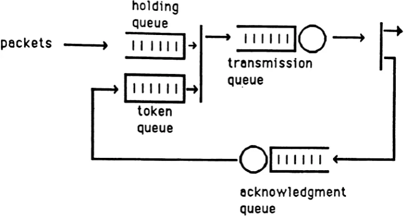
Figure 1 - Single Sliding Window Flow Control

Packets arrive at the holding queue. If there is a token available at the token queue, a packet

takes the token and proceeds to the transmission queue. Upon service completion the packet

leaves the system and the token joins the acknowledgment queue. After completion of its service. the token joins the token queue. Packets that arrive at the system when the token queue is empty are forced to wait in the holding queue. The number of tokens is set equal to the maximum window size.

In order to represent the window flow control in a simple manner, we make use of the

tol-lowing two symbols

1111111'-'

1111111111-+

(We note that these symbols are similar to those used in Fdida, Perras. and Wilk [19]). The

join symbol depicts the following operation: when both queues contain a customer each. the

two custo·m.ers instantaneously depart from their respective queues and merge into a single

customer. The split symbol depicts the operation where a customer arriving at this point is

split into two entities.

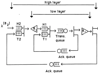
Now, let us consider the above single-hop communication link with two layers or nested sliding

window flow control and packet fragmentation/reassembly, as shown in Figure 2.

h1 gh layer

'low leyer

~---i

[B 2]

H2

H1

.

)..

~

_~

_{-, "'U-,}

~ ,...(1~""i"i711

_~-+

I

r

_.1JI]O

_--+

...-.... IT:!TI

IT:!TI

T

rens.

T2

T 1

Queue

~---O@I

Ack. Queue

O@I~---"'"

Ack. Queue

Figure 2 - The Model for th~ Nested Two-Layered

Sliding Window Flow Control

~

_--+

fregmentot

ton

reassembtq

The fragmentation symbol indicates the operation where a packet upon arrival at that point is

split into 8 subpackets. This operation is assumed to take zero time. The reassembly symbol

indicates a buffer where subpackets watt. When the 8th subpacket arrives, all the B sub-packets are instantaneously assembled into a single packet which is released immediately

For presentation purposes, we shall refer to the outside window flow control in Figure 2 as the

high layer, and to the inside window now control as the low layer. Packets arrive at the high

layer according to a Poisson process with rate A. An arriving packet is immediately frag-mented into B2 high layer packets. Each of these packets requires a token from the token

queue T2 in order to enter the low layer. Those high layer packets for which there is no token

available are forced to wait in the holding queue H2. Upon entry to the low layer. a high layer

packet is immediately fragmented into 8, low layer packets. Each of these packets is 1hen

subjected to window now control using token queue T1. They are then transmitted to the

re-ceiver one at a time. An acknowledgment for a low layer packet is generated immediately

upon receipt of the packet. High layer packets are acknowledged upon receipt of Bt low layer

packets comprising the original high layer packet Let W2 and Wt be the window size for the

high and low layer respectively.

We assume that packets arrive in the order in which they were sent, as would be the case in

a virtual circuit protocol. The transmission time is modelled as a single server queue with

exponentially distributed server time. Retransmission of packets is ignored. assuming that the

mean transmission time measures average time to successfully deliver a packet. We also

assume an infinite buffer at layer 2, and sufficient buffer space at layer 1 to hold W28 ,packets.

in addition to the transmission time These service delays have been ignored as we wish to

focus on the interaction between the sliding window now control and packet

fragmenta1ion/reassembly. These delays can be easily incorporated approximately seeing

that the model is analyzed using a hierarchical decomposition method.

Although the above described model has only two layers of sliding window control, it is of

sufficient generality to demonstrate the method of analysis proposed here. The goal is to

re-duce an arbitrary number of nested layers of sliding window control to a single server queue

which represents the performance characteristics of the nested layers. This is done in a

hi-erarchical manner. We first analyze the low layer, as shown in Figure 1,in order to construct a flow-equivalent queue. (This equivalent queue is obtained assuming a Poisson arrival

pro-cess. Upon arrival, a packet is immediately fragmented into 81 subpackets.) Then, in Figure

2, we replace the low layer by its equivalent queue, thus obtaining a queueing model similar

to the one shown in Figure 3, where the transmission queue represents the equivalent queue.

holding

_AX

X

n

R

(8]

Queue

-~~

I I I I I

IIO-~-+

1-+

~

I

1-+

)

II

n

trensrm

5S1

on

reessembly

II

I

n

I1-+

Queue

buff

er

token

W

eck

Queue

_Queue

011

I I I I I

Jl

_A

n

_A

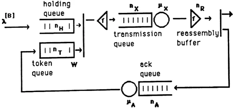
Figure 3 - The Model of a Sliding Window Flow Control

With Packet Fragmentation and Reassembly

Next. we reduce the network in Figure 3 to a single queue, which will represent the

charac-teristics of the oriqinal network. Ifthere is another protocol layer above the two depicted in

Note that unlike the methodology in [12] and related papers, this study does not use a

state-dependent service rate in the equivalent queue. Given exponential transmission times, each

equivalent queue will be of the Erlang type.

It is evident that in order to be able to tackle any number of nested layers of sliding window

now control we need to be able to construct a flow equivalent Queue of the Queuing system

shown in Figure 3. This is taken up in the following section.

III. Reduction to a Single Queue

Let us consider the model shown in Figure 3. Arrivals are in batches of B. The inter-arrival time between two batches is exponentially distributed with mean 1/J.. The window size is W.

When a packet goes through window flow control it is fragmented into f packets. We shall

refer to the packets in the holding queue as high layer packets, and the fragmented packets

inside the window flow control as low layer packets. The service times at the transmission

queue and the acknowledgment queue are exponentially distributed with parameter J..Lx and

J.LA respectively.

Let us define the following notation:

nH: number of high layer packets in holding queue

nr: number of tokens in token queue

nA: number of tokens in acknowledgment queue nx: number of lower layer packets in transmission queue

nR: number of lower layer packets in reassembly buffer ns: number of high layer packets undelivered.

(i.e .. the number of packets"in the system"). 1

ns= nH

+ ,

+

Given the triple _{(ns• nAt nR)} other quantities above can be calculated using the following

re-lations:

nx= fmin(ns. W - nA) - nR'

The triple (ns ,

n

n

letPIJ,Irbe the probability of finding the system in state (iJ,k) in steady state. The steady state

probability balance equations which determinePIJ,Irare:

lpooo -

ns

=

+

=

=

(A.

+

=

0< ns <

(A.

+

(A.

+

=

+

=

(~

+

+

=

+

=

(A

+

+

+

j = 1,2, ..., W - 2 k = 1,2, ..., f - 1

(A

+

+

=

=

+

(1)

(A

+

+

(A.

+

=

+

+

=

(A.

+

+

+

+

(A

+

+

=

+

+

j=1 ,2, ...,W-2 k=1.2 .... ,f-1

(A

+

+

+

(A.

+

=

+

It is desired to reduce the sliding window controlled network of Figure 3 to a single server

queue, and to that end we look at the probabilities

Pit

P,is the probability of having i high layer packets in the entire system. We will work from the

rate equations governing Pi' in order to construct this equivalent queue.

The rate equations governing PI are obtained by summing all of the rate equations (1) with

i

as a subscript on the left hand side. These equations are, (with like terms on left and right

hand sides cancelled),

0<;<8 .

W-1

A.Po

=

W-1 W-1

APi = JLxL PI+1J.f-1 - JLx

I

j=O j=O

W-1 W-1

APi

=

+

i

~

J=O j=O

(3)

W-1

We see that the summation

L

j:O

of being in those states from which an immediate transition to a state with one less high layer

packet in the system is possible when there are ipackets in the system. (The numberofhigh layer packets in the system only decreases when the final fragment of an original high layer

packet completes transmission. This only occurs when the number in the reassembly buffer

isf - 1 ).

It is desirable to have a set of rate equations for Piwhich do not depend upon the "internal"

parameters of the lower layer,

n

n

reas-sembly buffer population can be eliminated by making the assumption (for

i

>

(4)

for each pair1<,1<' E {O,1, ...,f - 1}. Assumption (4) states that it is equally likely to find any of

as nA

_<

spent with k in the reassembly buffer, (given that a packet is in transmission), is

1/11"

(In fact, while it is true that

00W-1 00W-1

I I

=

I

1=1)=0 ;=1j=O

(4) is not true: however, (4) proves to be an adequate assumption).

Using assumption (4) and (2) we have

'-1 W-1 W-1

Pi

=

+

I

+ ,

k=O j=O J=O

thus

W-1

I

j=O

(5)

(5) shows another quantity that proves pivotal in the analysis of the sliding window protocol:

p;,W,O' is the probability that all tokens are in the acknowledgement queue, and i high layer

packets are in the system. Define B;as the conditional probability of having all the tokens in

the acknowledgment queue given

i

Combining (5) and (6), we have

Bj =

Pi,W,O

P,

W-1

I

=

j=O

W-l

Substituting this expression for

L

j-a

set of rate equations for a bulk arrival queue with state dependent exponential service rate

J.Lx

-,- (1 - 8,).

The values a; can be calculated from the solution to the rate equations (3). There is no known

closed form solution to these equations, thus the solution must rely upon a numerical

tech-nique. Other authors who have used a flow equivalent server methodology to model sliding

window protocols use an approximation procedure to generate the

e, ,

=

>

of the transmission and acknowledgement queues when there are i packets in the closed

network. Since this throughput is equal to Ilx(1 - a), the computation of

a,

observed empirically that the results of this approximation are not good for a bulk arrival

system, while they are satisfactory for Poisson arrivals, (see Fdida, Perros, Wilk (19)).

This study takes another approach to simplifying this system. We shall replace the state

de-pendent service rates

1J.;

a

some sense, an average of the state dependent rates. This results in a fairly simple

approx-imation of the original system.

0.01

e.ee

0.07

0.015

0

LOS

0.01 0.OS

12 15 18 it a

i

high loyer packets in system

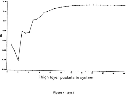
Figure 4 -B,vs.i

We observe that the values tend towards a constant as i gets large. This behavior was

ex-hibited for every choice of parameter values of the system.

Let us refer to the settling down of a,to a constant as ; increases as a state-asymptotic prop-erty. (This is to distinguish from time asymptotic behavior). That all systems examined show

this behavior is not surprising. The state transition structure of the model is aperiodic. When

there are a large number of packets in the system, the system will behave much like a closed

model with W tokens circulating. in that erich token returning to the sending station will find

a packet waiting. As the holding queue is being depleted. the tokens will be continuously

moving through the system and we would expect that the distribution of the tokens between

the acknowledgment and transmission queues will reach a statistical equilibrium. Let us

de-note the state-asymptotic value of

a,

this point. since the holding queue has been empty. the sending station will have had a chance

to "stockpile" some tokens. and thus the probability of having all tokens in the

acknowledg-ment queue will be relatively low. (The state i = B can also be reached by a transmission

completion with B

+

this event is less likely than arrival to an empty system.)

To construct a single queue approximation to the model under study with state indepehdent

service rate, we would like to find a value 8 which is an average of the

e;

Let us look at estimating Bf)t'l' the upper bound on

a.

Figure 5.

"x

...--01111111

J1

_A

"A

Figure 5 - Closed Model Used in Approximation Procedure

The rate diagrClm for this closed network is shown in Figure 6. for the case where' = 3 and

~=O

n

_R

-:

1

_n

R

-=2 )

Jl

_X

X

nA=O

0

0

Q/PX

n~~A

T

Jl

_A

Jl

A

T

Jl

_X

0

J1

X

)

.A

,

~

T

Jl

A

Jl

_X

T

Jl

_A

Jl

_X

n

A

: 2 0

0

\ , 1

Jl

_A

J!x

t

Jl

A

J1

_x

n

_{A = 3 0}

~O

T

Jl

_A

n

A

0

Figure 6 - Rate Diagram of Model Shown

in Figure 5 for W

=

Take for the state of the closed system the pair (n_{A ,}nR ) . Denote the probability of state U.k)

by

YI.It-Sin~e there are Afinite number of states in this model, the state probabilities of this system

are rather easily solved for. It seems that the probabilityYw.o should be a good estimate of

80t'l' as the original system under saturation behaves much like a closed network; however. it

turns out thatYw.o over-estimates Bot"for every choice of parameters examined.

An explanation for this discrepancy comes from comparing the nature of the closed system

to the original. Note that in the original system each transmission completion when

sys-tern there is no explicit value of n_{s .} Itis assumed that n_s is "Iarge", and that the number in the acknowledgment queue is increased at the rate at which transmission completions occur

when nR= , - 1, and decreased at the rate at which acknowledgment completions occur. Thus

the closed model estimates for large

n

+

n

n

+

p;"'J,t-1were equal, then the closed model would accurately predict the probability distribution

of the acknowledgment queue for large n_{s ;}however, in general these probabilities are not equal.

If we look at the state asymptotic behavior of the probabilities Pi' we note that the value of

Pi~lIP; tends to a constant ratio as igets large. (see Figure 7).

'.1

1.2

1.1 1.0

0 0•8

:;J

~o.e

;0.7

.D0 • 8

o

-OD.5

o

~

a..

0.2

0.1

• • II 1$ , . II " 17

Number of high level packets in system

Figure 7 -

P;, tiP;

This phenomenon is observed for all of the test cases run. We thus post that for; large

for some Yoo E (0.1). A formula for Yon comes from summing the aggregate rate equations (3)

for i

=

+

N+B W-1

A L PI

=

I=N+1 j=O

From (7) and (assuming Nis large) assumption (8), (9) becomes, (after simplification),

(9)

B

= 1 - - , { - 1-yoo

(Jlx/fJ Y~(1 - Y(0) .

We see that assumption (8) implies the existence of Boo' since the right-hand side above is independent ofN. We thus have an equation relating Booand Yoo

B

1 - - , { - 1-yoo

Boo

=

y~(1

Another equation relating a_oo and Yoo is obtained from an analysis of the closed network,

(Fig-ure 5). We have already seen that empirical evidence indicates that there is a constant ratio between state probabilities for large

n

ac-knowledgment queue in the closed model in order to reflect more accurately the true

dy-namics of the system. Since the only service completions which result in a token entering the

acknowledgment queue are those which occur when

n

at which transmission completions occur in these states by YooJlx, and leave the other service rates alone.

The probability balance equations for this modified system are:

Yoo JlXY W- 1,f- 1

=

=

W - 1

+

n

(-1

'YooIJ. XYj,f- 1

=

k=O

J..LXYj,f-2 = (J..LA

+

J1XYj,k = (J.l.A

+

(-1

'YooIJ.XYO,f- 1

=

k=O

J.l.XYO,f-2

=

JI.XYO,k

=

=

(11)

Equations (11) can be solved by noting that the closed network on which the rate equations

are based can be cast as a Coxian server with a state dependent arrival rate. Marie, [20], has

developed an algorithm for solving for the state probabilities of such a queue.

Let us see how the closed network can be described as a Coxian server with state dependent

arrival rates. Let nc

=

queue, (including the high layer packet in service). Arrivals to the transmission queue occur

at rate J..LA whenever the acknowledgment queue is not empty, thus the state dependent arrival

process to the transmission queue, denoted by A(n_c)is given by

_ {JlA, nc = 0,1, ...,W-1

A.(nc) -

°

>

The transmission server can be thought of as a Coxian-f server of high layer packets. A high

layer packet beginning service at the transmission server requires f sequential exponential

service phases before completing service. In the model with modified rates, (i.e. (11)), the first

, - 1 service phases have rate IJ.x and the last phase has rate '100 IJ.xo Yw.o •the probability of

having arl tokens in the acknowledgment queue in the closed model, is equal to the probability

that n_c

=

Using the solution from (11) for Yw,o as an estimate of Boo together with (10) gives us two

re-lationships betweenBoo andYoo' Solving for the pairBoo' Yoowhich simultaneously satisfies both

relations resulted in a consistent under-estimate of Boo; however, this under-estimate proved empirically to be a fairly good choice for

a.

sol-ution to (10) and (11). Thus, the following algorithm proves to give a good value for 8.

Approximation Algorithm

1. Let }'~= 1. Solve (11) for 8

00,

2. Use the value of800 from 1) to calculate a new Yoo ' using (10).

3. Using 'Yoo from 2), calculate a new Boo from the closed network equations (11). Use this

value ofa~ for

a.

The approximation algorithm gives a good estimate for the average service rate of high layer

packets,

~x

expo-nentially distributed transmissions to deliver a high layer packet. The transmission time for

the high layer packet thus has an Erlang-f distribution. In the approximation procedure, we

used an Erlang-h server with mean service rate

Il;

network as seen by the higher layer.

The number of stages, h, in the approximate Erlang server is determined as follows. If f is 2

or 3,h

=

=

in the approximation algorithm against exact solutions computed by Neuts' matrix-geometric

procedure, [21]. For anyf> 3, h= 3 is used. Since the sliding window mechanism introduces variability into the effective delivery time distribution beyond that of the transmission time

distribution, less than f stages are used in the approximate model, since the Erlang-k family

of distributions has increasing variance as k decreases. The exception to this rule Is when

f= 2. In this case the Erlang-2 distribution and the exponential. or Erlang-1. gave comparable

results. The number of stages In the approximate model is limited to three, since the Erlang-k

distributions become less distinct as k increases. It is hoped that using no more than three

Limiting the number of stages in the approximate Erlang server also helps to keep the

com-putational burden of the approximation scheme down when more than two nested layers of

sliding window protocol are analyzed. Consider the network of Figure 8(a). This network has

three layers of sliding window protocol. Analyzing the performance of this network

hierar-chically, we would first reduce the lowest layer to a single exponential server. We use the

approximation algorithm to compute the service rate of this server, analyzing the lowest layer

model with arrivals at rate

AB

B

network of Figure 8(b). Now we use the approximation algorithm to reduce the lowest layer

of sliding window protocol in this network, using an arrival process of rate

AB

=

The network of Figure 8(c) appears to be a model which we have not yet considered. It differs

from the model of Figure 3 by having an Erlang rather than an exponential server. From a modelling point of view, however, these two networks have the same structure. In the model

of Figure 3 f exponential services must be completed to deliver a high layer packet. From the

point of view of the higher layer, the fragmentation and re-assembly of the lower layer are

invisible; the higher layer sees the delivery as an Erlang t, (fexponential times on per

frag-ment). In Figure 8(c), B2 Erlang services must be completed to deliver a high layer packet.

Since one Erlang-h service is composed of the sum of h exponential random variables,

deliv-ery of a high layer packet in the model of Figure 8(c) takes hB2exponential delays; thus the

model of Figure 8(c) is equivalent to the model of Figure 3 when f = hB2• Casting the problem

in this form, we can reduce the network of Figure 8(c) to a single queue using the

approxi-mation algorithm.

We now see why keeping the number of Erlang stages in the approximation server small is

~---

OE

Jl

A

1

(e) - Orlg1nel model

~----

OE ....

(

-Jl

_A2

" " " - - - 0 E

Jl

A

1

(b) - lowest 1evel

reduced

...-.---- OE

...

Jl

A

1

(c) - two lowest levels

reduced

Table 1 • Data Set Parameters for Validation of Queueing Model Shown In Figure 3

Data Set

Number % of maximumlBflJ.lxas Batchsize

Window size

Frag

1 22% ₃

₂

₂

2

₂

3 20% _{3 4}

₂

4 20% _{3 15}

₂

5

₂

6 17% 3 4 4 .23

7 24% ₃

₂

8 35% ₈

₂

₂

9 32% 8 4

2

10 48% 8

2

11 79% 3 2

2

12 67% _{3 4}

₂

13 62% 3 8

2

14 70% 3

2

15 62% ₃ 4 4 .63

16 60% 3 8 4 .63

17 69% 3

2

18 61% 3 4 10 .63

19 80% 6

2

2

20 67% 6 4

2

21 62% 6 8 2 .83

22 96% 6

2

5

23 81% 6 4 5 1.25

24 93% 3 4 2 .94

25 85% 3 8 2 .94

26 98~o 3

2

27 84% 3 4 8 .75

28

29

2

30 82% 5 8

2

31 86% 5

2

5

IV. APPROXIMATION RESULTS

The approximation algorithm was evaluated for 32 data sets of networks with the structure of

Figure 3. The parameters for these data sets are shown in Table 1. In each case the

ap-proximate results were compared to exact solutions obtained numerically. The numerical

procedure for these models required working with matrices of the order of f BW, so there is

a practical limit on the range of parameters which could be tested. Within these limits, the

system utilization, (the second column of Table 1 shows the offered load as a percentage of

the maximum possible throughput), the window size, f, and the ratio of high layer packet

transmission time to acknowledgment transmission time. (

~.

)IIlA

The numerical procedure used was Neuts: matrix-geometric algorithm, [21]. Due to the highly

regular structure of the rate equations (1), considerable computational efficienciescan be

ef-fected. In a straight-forward appllcation of the matrix-geometric algorithm, a matrix of

di-mension fBW would need to be inverted. This matrix has a block structure. and its inverse

can be evaluated directly in terms of the inverse of anf\Nsized block. The smaller block also

has a regular structure, and its inverse can be written without recourse to a numerical

pro-cedure. The algorithm was written in PASCAL, and the abstract data typing features of that

language facilitated the block structure representation of the rate matrix.

Figure 9 shows the relative error in mean number of high layer packets in the system vs. the

predicted probability that the acknowledgment queue is full. The probability of having the

acknowledgment queue full is a measure of how far from a true Erlang distribution the

trans-mission time distribution will be. The percent errors are fairly low. In addition to the errors

introduced by not having an Erlang transmission distribution, there are also errors due to

approximating a system with f> 5 by an Erlang-3. Figure 10 shows the relative error in

pre-dicted mean vs. probability that the acknowledgment queue is full, for those data sets where

, =

many data points were calculated). In this case. we see that the errors are roughly correlated

0.4

0.3

0.2

8

6

2 .

o

_ _

0.0

4

10

~

E

...

.., c

.,

_....

~

Q) '

-L. 0

t:

Q)

probebillty eck Queue full

Fi gure 9 - Rel at1ve Error

01

the Mean Number

of

Hi gh

Leyer

Packets vs.

Probability

Ack.

Queue

is

Full

0.3

02

0.0

c

4

E~

₃

2

_E

..,

CD ~

₁

...-

c:

Q)

L.

probebility eck Queue full

Fi gure 10 - Re let

i

ve Error of the rteen Number of

While errors due to Erlang "fit" problems cloud the picture. it is generally true 'hat for a given

f.

'~

)/II

performance, having relative errors from 5% to 10%. This observation matches that of

pre-vious studies, (15].

Table

2

Pi

maximum relative error for states with probability greater than 0..001 are shown. The results

are fairly good. In Table 2 we also show the relative error at the value ofi for which the

maximum absolute error was observed. and the absolute error for the value of i where the

maximum relative error was observed.

Figure 11 shows the predicted and actual PI probabilities for data set 23, which was one of the

poorest predictions, having a maximum deviation of 0.05.

6.0e-2

5.0e-2

exact

::n

4.0e-2

predi cted

+J

.0

3.0e-2

CD

.c 0

L.

2.0e-2

Q.

1.0e-2

o

number of hi gh

layer packets

Figure 11 - Predicted vs. Actual Probability Distribution

Table 2 • Predicted vs. Actual

Pi

Data Set Maximum Corresp. Maximum Corresp.

Number Absolute Error reI. error rel.error * Abs. Error

1

2 8.45e-03 12.1 % 12.1 % 8.45 e-03

3 6.2 e-OS 0.008% 0.1% 4.7 e-Q6

4 1.8 e-10 0.0% 0.0% 1.8 e-10

5 7.0 e-Q4 1.4% 14.1% 4.0 e-04

6 4.3 e-Q4 0.8% 13.5% 3.8 e-D4

7 1.5 e-03 2.0% 34.8% 3.6 e-D4

8 1.8 e-03 4.9% 4.9'% _{1.8 e-03}

9 1.6 e-04 0.020/0 0.48% 3.2 e-D5

10 6.5 e-04 1.3% 10.4% 1.1 e-04

11 7.0 e-03 3.1 % 19.10/0 2.2 e-04

12 1.4 e-02 3.7% 8.1 % 9.5 e-05

13 4.1 e-03 1.0% 1.8% 2.0 e-04

14 9.5 e-Q3 3.0% 17.1 % 1.9 e-Q4

15 4.0 e-03 1.0% 26.7% 2.8 e-Q4

16 4.4 e-03 3.4% 26.4% 3.2 e-Q4

17 1.3 e-03 3.90/0 37.9% 3.9 e-Q4

18 6.6 e-03 5.10/0 46.3% 5.4 e-Q4

19 5.0 e-03 10.0% 10.0% 5.0 e-D3 .

20 1.4 e-03 4.0% 5.25% 1.5 e-03

21 6.1 e-03 1.5% 2.4% 2.3 e-Q4

22 3.5 e-03 7.2% 9.5% 1.4 e-D3

23 5.0 e-02 20.3% 20.3% 5.0 e-02

24 9.2 e-03 11.2% 18.3% 1.9 e-Q4

25 1.3 e-02 7.6% 11.0% 1.2 e-04

26 2.1 e-03 7.4% 9.4% 9.7 e-04

27 7.9 e-03 4.6% 15.5% 1.6 e-04

28 3.0 e-03 3.9% 22.7% 2.5 e-04

29 1.3 e-02 10.4% 10.4°/0 1.3 e-02

30 1.4 e-02 6.8°10 6.8°10 1.4 e-02

31 4.8 e-03 3.2% 4.7% 1.8 e-03

32 2.1 e-03 1.4°/0 6.3°10 6.5 e-OS

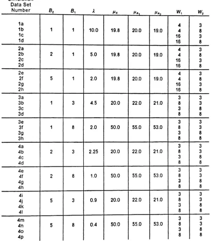
Table 3 • Simulation Data Set Parameters for Validation of the Queueing Model shown in Figure 2

B,

_I,

1a _{4 3}

1b 1 1 10.0 19.8 20.0 19.0 4 8

1c _{16 3}

1d _{16 8}

2a _{4 3}

2b 2 1 5.0 19.8 20.0 19.0 4 8

2c _{16 3}

2d _{16 8}

2e 4 3

2f 5 1 2.0 19.8 20.0 19.0 4 8

2g

2h 16 8

3a 3 3

3b 1 3 4.5 20.0 22.0 21.0 8 3

3c 3 8

3d 8 8

3e 3 3

3f 1 8 2.0 50.0 55.0 53.0 8 3

3g 3 8

3h 8 8

4a 3 3

4b

2

4c 3 8

4d 8 8

4e 3 3

4f 2 8 1.0 50.0 55.0 53.0 8 3

4g 3 8

4h 8 8

4i 3 3

4j 5 3 0.9 20.0 22.0 21.0 8 3

4k 3 8

41 8 8

4m

4n

0.4

40 3 8

4p

Simulation Data Set

Multi-layer Simulation vs. Approximation Results

Above we compared the results of the approximation algorithm of Section III to exact results

for a model with the structure of Figure 2. The comparisons of the approximate results to

exact results assumes that the transmission queue is an exact representation of the lower

layer network, and thus allows us to evaluate the approximation algorithm apart from errors

in the lower layer approximation. We next evaluated the performance of the hierarchical

method.

We performed the hierarchical reduction for 36 examples with the structure of Figure 2. In

each case the approximation algorithm was used to reduce the lower layer sliding window

control shown in Figure 1 to a single queue, assuming arrivals at the rate AB2. In this case the

lower layer approximation is simplified since there is no fragmentation inside the lower layer

window flow control. The resulting approximation queue was then used as the transmission

queue in a network with the structure of Figure 3, and this latter network was analyzed by the

approximation algorithm.

The data set parameters used are shown in Table 3. We attempted to use enough data sets

to examine the various possible relationships between W1, W2, B1 •and 82 .

Due to the large state space associated with an exact probabilistic model of Figure 2, we are

not able to generate exact solutions against which to compare the approximation results. We

thus constructed a simulation model of the network in Figure 2, with the rates, window sizes,

and amount of fragmentation as parameters. We used the results from a simulation model

as a basis of comparison for the approximation results. For each data set in Table 3, a

num-ber of independent replications of the simulation were run. Each replication began with no

packets in the system, and all tokens at both layers in the token queue. Each replication was

terminated after 500 high layer packets were delivered. We calculated the mean number of

high layer packets in the system for each replication, and from these values calculated an

approximate 95% confidence interval for the mean number of high layer packets in the

The comparison of the simulation mean number of high layer packets in the system and the

predicted mean number from the hierarchical approximation is shown in Table 4 We see that

with the exception of cases 3a. 3c, 3f, 3h, 4a, and 4c, the approximate means lie within the 95%

confidence intervals.

We also used the simulation data to construct point estimates of the probability distribution

of the number of high layer packets in the system, along with the associated approximate 95%

confidence intervals for these estimates. Figure 12 shows a comparison of the probability

distribution of high layer packets in the system obtained using simulation against the

proba-bility distribution generated by the approximation algorithm. Figure 12 is for case 4m, and

was selected as being typical.

0.08

20

10

number of hi gh leyer

packets

0.00

o

0.06

-m-

:n

...

sVnul~tion

~

....

~

....

.c

0.04

.,

D

0

s;

c..

0.02

Figure 12 - Comparison of Simulation and Approximation Probability

Distributions of the Number of High Layer Packets for Data Set 4m

We also experimented with a state-dependent now-equivalent server approach. developed by

Fdida. Perros. and Wilk. (19). The authors developed this procedure assuming single Poisson

arrivals at rate

J.:

procedure agalns samp e

Table 4 • Comparison of Approximate and Simulation Means for the Data Sets Given In Table 3

Data Approx. Simulation 95% conf.

Set mean mean interval

1a 1.64086 1.609 ±0.3516

1b 1.182 1.1778 ±0.1997

1c 1.4297 1.445 ±0.2807

1d 1.0355 1.001 ±0.1308

2a 2.7365 2.3068 ±0.5234

2b 1.8230 1.7338 ±0.3324

2c 2.4025 2.033 ±0.4543

2d 1.6075 1.4247 ±0.2428

2e 6.2412 6.108 ±1.610

2f 3.9034 4.1997 ±O.8466

29 5.5368 5.4561 ±1.4297

2h 3.5031 2.8488 ±0.6891

3a 4.0051 3.2045 ±0.4435

3b 1.9267 1.7681 ±0.2595

3c 3.9699 3.2013 ±0.4440

3d 1.9115 1.7655 ±0.2593

3e 0.5351 0.5244 ±0.O286

3f 0.4347 0.4127 ±O.O194

3g 0.5351 0.5245 ±0.0286

3h 0.4347 0.4127 ±0.O194

4a 6.5422 5.6219 ±O.8189

4b 3.1004 2.7855 ±0.4104

4c 6.4776 5.6043 ±O.8200

4d 3.0694 2.7749 ±0.4123

4e 0.8414 0.8300 ±0.0724

4f 0.6787 0.6452 ±0.0505

4g 0.8414 0.8300 ±0.0724

4h 0.6787 0.6452 ±0.OS05

4i 11.416 13.693 ±3.1462

4j 6.6247 7.4186 ±1.4554

4k 14.001 13.675 ±3.1474

41 6.5432 7.3887 ±1.4545

4m

4n 1.4108 1.3066 ±0.1541

40

The method performed well with single arrivals, though errors were slightly higher for both

predicted mean and predicted distribution compared to the algorithm in this paper. For

batched arrivals, (8

>

state probabilities were monotonically decreasing, and did not reflect the true shape of the

distribution. The relative errors for the mean number in the system exceeded

250~

cases.

An explanation for the poor performance of the flow-equivalence methodology with batched

arrivals is the assumption inherent in the technique that the service rate with n packets in the

system is the service rate of a closed system in steady-state with min (n,W) packets present.

With batched arrivals this instantaneous steady-state assumption is not warranted.

v.

In this paper we have presented a new procedure for approximating the behavior of a single

hop network with multiple layers of sliding window flow control. The method differs from most

previous research presented in the published literature in that it explicitly takes into account

the fragmentation of packets which occurs in actual systems. The procedure was compared

to exact numerical solutions, and found to perform well.

We see particularly that for systems with batched arrivals that the state asymptotic approach

yields better results than procedures based on

a

flow-equivalent server technique assumes an "instantaneous steady state" behavior of the

net-work, that is, the network with a given population behaves like a closed network in steady

state with that population. This technique is successful in the models where the state does

not change dramatically in anyone instantaneous transition. This is clearly not the case in

systemswith batched arrivals.

The procedure is easy to implement, and easy to solve on a computer. Its speed makes it

feasible to think of including the procedure in an interactive network designer expert system,

The procedure reports its results as the service rate and number of exponential service stages

of a queue. This should make it a useful add-on to general purpose queueing network solution

software packages. These packages typically cannot handle the special features of a sliding

window protocol. By reducing the portions of the queueing network which have sliding

win-dow control to a single queue, the procedure approximates the sliding winwin-dow sub-net by a

REFERENCES

[1J ~.S. Tanenbaum, Computer Networks, Englewood Cliffs NJ: Prentice-Hall, Second

Edi-tion, 1988. '

(2] M. Gerla and L. Kleinrock, "Flow Control: A Comparative Survey," IEEE Trans. Com-mun., Vol. COM-28, April 1980

(3] M.C. Pennotti and M. Schwartz, "Congestion Control in Store and Forward Tandem Links," IEEE Trans. Commun., Vol. COM-23, December 1975.

[4] A: Chaterjee, N.D. Georganas, and P.K. Verma, ..Analysis of a Packet Switched Network with End to End Congestion Control and Random Routing," IEEE Trans. Commun., Vol. COM-25, December 1977.

[5] J. Labetoulle,. G. Pujolle, and N. Mikou, ..A Study of Flows in an X25 Environment," in Flow Control In Computer Networks, J.L. Grange and M. Gien, Eds, NY: North Holland, 1979.

[6] M.Reiser, itA Queueing Network Analysis of Computer Communication Networks with Window Flow Control," IEEE Trans. Commun. Vol. COM-27. August 1979.

[7] S. Lam, "Queueing Networks with Population Size Constraint," IBM Journal of Res. and Develop., Vol. 21, No.4, 1977.

[8] A. Thomasian and P. Bay, "Analysis of Queueing Network Models with Population Size Constraints and Delayed Blocked Customers," in Proc. 1984 ACM SIGMETRICS Confer-ence on Measurement and Modelling of Computer Systems,

a

[9] K. Goto, Y. Takahashi, and J. Hasegawa, IIAn Approximate Analysis of Controlled Tan-dem Queues," in Proc. of the Int'l Seminar on Modelling and Performance Evaluation Methodology, Paris, 1983.

[10] I.F. Akyildiz, "Performance Analysis of Computer and Communications Networks with local and Global Window Flow Control," INFOCOM '88, pp. 400-410.

[11J L. Kleinrock and P. Kermani, "Static Flow Control in Store and Forward Computer Net-works," IEEE Trans. Commun., Vol. COM-2S, February 19S0.

[12J M. Reiser, "Adrnlsslon Delays on Virtual Routes with Window Flow Control," in Perf. of Data Commun. Systems and Their Applications, G. Pujolle, ed., NY: North Holland, 1981.

[13J A. Thomasian and P. Bay, "Performance Analysis of Window Flow Control for Multiple Virtual Routes," Proc. IEEE INFOCOM '84, San Francisco, April 9, 1984.

[14J O. Gihr and P.J. Kuehn, "Comparison of Communication Services with Connection-or-iented and Connectionless Data Transmission," in Proc. Int'I. Seminar on Computer Networking and Performance Evaluation. Tokyo, September 18-20. 1985.

[15] G.

A.A.

Minneap-olis, 1983.

[16] M. Schwartz, IIPerformance Analysis of the SNA Virtual Route Pacing Control," IEEE Trans. Commun., Vol. COM-30, Jan. 1982.

[18) M. Murata and H. Takagi, "Two-Layer Modeling for Local Area Networks," IEEE Trans. Commun., Vol. COM-36, Sept. 1988.

(19) S. Fdida, H. Perras, and A.Wilk, "Semaphore Queues: Modelling Multi-Layered Window Flow Control Mechanisms," IEEE Trans. Commun., (to appear).

(20] R. Marie, "Calculating Equilibrium Probabilities for1(n)/CIc

/1/N

of Performance '80, Toronto, 1980.