Adsorption of Amphoteric and Nonionic Polymers on Model Thin Films

(1)

ABSTRACT

SONG, JUNLONG. Adsorption of Amphoteric and Nonionic Polymers on Model Thin Films. (Under the direction of Prof. Orlando J. Rojas).

Understanding the adsorption behaviors of polymers from solution is critical in

applications such as fiber processing, specifically in the development of fiber bonding and lubrication. Therefore, in situ and real time Quartz Crystal Microbalance and Surface

Plasmon Resonance were employed to monitor the adsorption of hydrosoluble polymers (including amphoteric and nonionic macromolecules) on ultrathin films of cellulose, polypropylene, polyethylene, nylon and polyethylene terephthalate.

The extent of adsorption of amphoteric polymers on cellulose (and also on silica) depended on the charge density of the polymer, the substrates and pH of the medium. More

importantly, the adsorbed amount exceeded that found in the case of simple polyelectrolytes. We hypothesized that this extensive adsorption is the result of a polarization effect produced by the charged substrate, which also determined the characteristics (thickness and

viscoelastivcity) of the adsorbed layers as well as bonding abilities.

Surface active polymers including diblock polyalkylene glycols and triblock

polymers (based on ethylene- and propylene- oxide) as well as silicone surfactants were used to study the formation of boundary layers that are relevant in fiber lubrication. Adsorption isotherms for the nonionic polymers followed a Langmuirian behavior in which the

hydrophobic effect was a major driving mechanism. It was concluded that surface-active molecules form robust self assembled (lubricant) layers that withstand high shear forces and

(2)

Adsorption of Amphoteric and Nonionic Polymers

on Model Thin Films

by

Junlong Song

A dissertation submitted to the Graduate Faculty of North Carolina State University

In partial fulfillment of the Requirements for the degree of

Doctor of Philosophy

Wood and Paper Science

Raleigh, North Carolina 2008

APPROVED BY:

_______________________________ ______________________________ Dr. Orlando J. Rojas Dr. Martin A. Hubbe

(3)

BIOGRAPHY

The author was born on May 6, 1974 in Yongchuan, Chongqing, People’s Republic of China. He grew up in his hometown until Fall 1994 when he joined Beijing Forestry University,

Beijing. He obtained a Bachelor degree in Chemical Engineering in 1998 and a Masters degree in Pulp and Paper Science in 2001, from the same institution and department. After

graduation, he worked as a process engineer for China International Engineering Co. Ltd (China BCEL) for three years. In July, 2004, he came to Raleigh to join the Ph.D. program in the Department of Wood and Paper Science in North Carolina State University.

(4)

ACKNOWLEDGMENTS

The author is immeasurably indebted to his major advisor, Dr. Orlando J. Rojas for his mentorship, advice and constructive criticism throughout the course of this research.

Special thanks are also extended to Ph.D. committee members, Drs. Martin A. Hubbe, Dimitris S. Argyropoulos and Kirill Efimenko. Drs. Juan P. Hinestroza, Tom Theyson and

Wendy Krause, are appreciated for giving valuable advice and ideas.

The author also wants to express his appreciation to Yun Wang, Yan Vivian Li and Hongyi Liu for warm discussions and for sharing thoughts and experiences. He is also in debt with

all his colleagues and friends in the Department of Wood and Paper Science, for their

assistance and encouragement and especially to the “Colloid and Interfaces” group members

with whom many memorable experiences inside and outside the university where shared. Finally, the author would like to state his appreciation to the US Department of Agriculture and the National Textile Center for funding the “polyampholytes” and the “boundary

(5)

LIST OF TABLES

Table 1.1. Comparison between QCM and SPR techniques (*)……….….22 Table 3.1. Characterizations of model surfaces………...77

Table 3.2. Comparison of the chemical composition from XPS and theoretical value…...85 Talbe 4.1. Synthesis of acrylamide-based polyampholytes and simple copolymers………..97

Talbe 4.2. Structure information of PAGs and Pluronics………98 Talbe 4.3. The maximum surface excess and area for each molecule calculated from Gibbs adsorption isotherm………...108 Table 5.1. Acrylamide-based polyampholytes (PAmp 2, 4, 8 and 16) and simple

polyelectrolytes (Cat and An). Note that in the case of the polyampholytes the %mol ratio cationic:anionic groups was kept constant at 5:4 and the molecular weight was approximately the same for all polymer samples………..117

Table 6.1. Structural information of polyalkylene glycols (PAGs) and Pluronics…………147 Table 6.2. Langmuir fitting parameters for adsorption curves of nonionic lubricants on PET surface after rinsing (irreversible adsorption)………160 Table 6.3. BET fitting parameters for adsorption curves of nonionic lubricants on PET surface after rinsing (irreversible adsorption)………....160 Table 6.4. Calculated hydrophobic numbers for tested nonionic polymers………. 166

(11)

LIST OF FIGURES

Figure 1.1. Polymer adsorption onto surfaces from solution. D is the thickness of adsorbed polymer layer……….3 Figure 1.2. Wet strength of paper treated with xanthated starch amine (XSA) having various tertiary amine and xanthate degrees of substitution (DS). The paper samples were prepared from unbleached kraft furnish treated with 3% XSA, oven dry pulp basis, at pH 7.0. Figure redrawn from reference 32………....6 Figure 1.3. Effect of macromolecular composition and pH on the tensile strength of polymer-treated bleached kraft fibers at 1000 µS/cm conductivity 25. Structures of polymers denoted as “PAmp 2, 4, 8, 16”, “Cat” and “An” can be seen with more detail in Chapter 3)…………7

Figure 1.4. Stribeck curve, displaying the different regimes of lubrication. Figure Redrawn from original source of Stribeck curve 40………...11

Figure 1.5. Proposed generalized friction map of effective viscosity plotted against shear rate. Figure redrawn from reference 42………...13 Figure 1.6. Proposed generalized friction map friction force plotted against sliding velocity. Figure redrawn from reference 42………...14 Figure 1.7. Proposed generalized friction map of friction force plotted against load. Figure redrawn from reference 42………..15 Figure 1.8. Schematic diagram of how the effective viscosity, elasticity and relaxation change with thickness of a lubricant film. Figure redrawn from reference 41………16 Figure 1.9. Lubricant molecules organized by shear. Figure redrawn from reference 49…..18

(12)

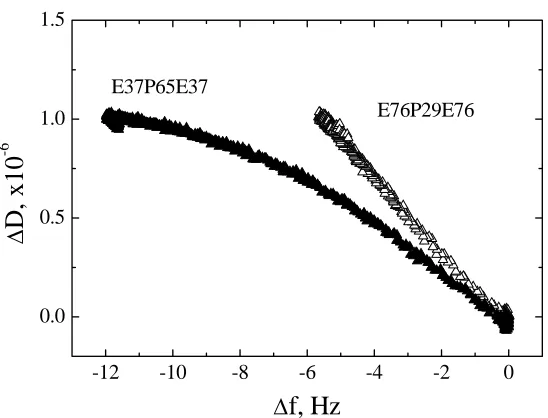
Figure 1.14. ΔD-Df profiles for polyampholyte adsorption on silica surfaces. The low charge density polyampholite (PAmp4) consisted of 5% cationic and 4% anionic groups while the high charge density polyampholyte (PAmp16) contained 20% of cationic and 16% anionic groups. The “cationic” polymer had a charge density of 5% (cationic groups)………..33 Figure 1.15. ΔD-Df profile of nonionic lubricants E76P29E76 and E37P65E37 as they adsorb onto PET surfaces before rinsing………...34

Figure 1.16. Comparison of adsorption kinetics of a perfluoropolyether lubricant (Fomblin ZDOL) on silver surfaces as measured by SPR and QCM . Figure from reference 84……...35

Figure 1.17. Decoupling water content through the combination of QCM and SPR measurements. The polymer used in this experiment is a cationic polyamide, with molecular weight of ca. 3 millions. Coupled water determined by this method was found to be 25%....37 Figure 1.18. Schematic of lateral force microscopy and twisting and bending motions acting on the cantilever………...39

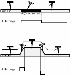
Figure 1.19. Lateral deflection of the cantilever from changes in surface friction (top) and from changes in slope (bottom)...40

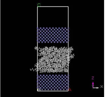
Figure 1.20. One line scanning profiles for the cellulose coated surface both in a Pluronic lubricant (E19P29E19, see Chapter 3 for detail) solutions and in air. P65 is the symbol of lubricant E19P29E19, which is a triblock copolymer with 19 EO groups at both ends and 29 PO groups in the middle. P65-1~P65-5 represent a series of ethanol solutions with the increase of ethanol concentration. Data contributed by project member Yan (Vivian) Li, from Cornell University………41 Figure 1.21. Sandwich-like layer to study the effect of shear in MDS. Top and bottom layers are Fe. Lubricant used was octane, C8H18, which can be seen between the two surfaces. The shear velocity for the two solid surfaces was set to 5 m/s. MDS results contributed by project member Hongyi Liu, from NC State………42 Figure 1.22. Animation of shear process for lubricant octane confined between two Fe surfaces. Shear velocity applied on both solid surfaces was 5 m/s. MDS results contributed by project member Hongyi Liu, from NC State………..44

(13)

Figure 1.24. Temperature profile of octane between two Fe surfaces. Shear velocity applied at both solid surfaces was set to 5 m/s. MDS results contributed by project member Hongyi Liu, from NC State………...46 Figure 2.1. Conformation of adsorbed polymers at interfaces for (a) homopolymers, (b) end-functionalized homopolymers, (c) Block polymers, and (d) polyampholytes……….60 Figure 3.1. AFM images of model films of (a) cellulose, (b) PP, (c) PE, (d) Nylon and (E) PET on silica wafers. Scanning size was 20 x 20　m for (d) and 2 x 2 　m for the rest…...76 Figure 3.2. XPS survey spectra for bare PP (a) and PE (b) films. Detail spectra (inset) for C1s BE region are included in each figure………..80 Figure 3.3. XPS spectra of cellulose model films (top). Detailed C1s spectra (bottom)…….83

Figure 3.4. XPS spectra of model (a) Nylon and PET (b) films. Detailed C1s spectra are seen in the insets………..84

Figure 3.5. Ellipsometric thicknesses of PP films obtained after different sequence times (larger sequence number indicates longer time and therefore larger )………... 87 Figure 3.6. Adsorption of a nonionic polymer (lubricant) (E37P56E37) on various model films . Adsorption isotherm was obtained by using the QCM-D technique………... 88 Figure 4.1. Molecular composition of monomers in random polyampholytes prepared by free-radical polymerization (DMAPAA, IA and AM)………96 Figure 4.2. Chemical structure of PAGs (a) and Pluronics (b)………97 Figure 4.3. Viscosity of polyampholytes (a) and viscosity changes against % charged groups of polyampholytes and simple polyelectrolytes (b)………...100

(14)

Figure 4.8. The radius of gyration of PAmp4 at different pH conditions………..105

Figure 4.9. Surface tension and CMC determination for bi-block polymer PAGs (a) and tri-block polymer Pluronics (b)………..107

Figure 4.10. Surface tension and CMC for the silicone surfactant LN336-100I…………..107 Figure 5.1. Molecular composition of monomers in random polyampholytes prepared by free-radical polymerization (DMAPAA, IA and AM)………..116 Figure 5.2. Frequency (top) and Energy dissipation change (bottom) curves for polyampholytes PAmp2, PAmp4, PAmp8 and PAmp16 as well as simple polyelectrolytes Cat and An at pH 4……….121 Figure 5.3. Frequency (top) and Energy dissipation change (bottom) curves for polyampholytes PAmp2, PAmp4, PAmp8 and PAmp16 as well as simple polyelectrolytes Cat and An at pH 7……….122

Figure 5.4. Frequency (top) and Energy dissipation change (bottom) curves for polyampholytes PAmp2, PAmp4, PAmp8 and PAmp16 as well as simple polyelectrolytes Cat and An at pH 10………...124

Figure 5.5. Comparison of thickness calculated by Sauerbrey and Voigt models for low (PAmp2, left) and high (PAmp8, right) charge density polyampholytes………..128 Figure 5.6. ΔD-Δf profile during adsorption on silica of polyampholytes and polyelectrolytes………. 130

Figure 5.7. Frequency change for different polyelectrolytes after reaching adsorption equilibrium……….132

(15)

Figure 6.2. Typical QCM f and D curves for an adsorbing nonionic polymer. Polymer sample was E76P29E76 in 0.0001% aqueous solution. Frequency (f) change (left axis) and dissipation (D) change (right axis) for three overtones (3, 5, 7) were recorded simultaneously. Flow rate was constant 0.1 ml/min………152 Figure 6.3. Equilibrium adsorption isotherms for nonionic lubricants adsorbed on PET surfaces at 25 °C before (a) and after (b) rinsing measured by QCM. The flow rate was constant at 0.1 ml/min………154 Figure 6.4. Equilibrium adsorption isotherms for nonionic lubricants adsorbed on PET surfaces at 25 °C before (a) and after (b) rinsing measured by SPR. The flow rate was kept constant at 0.1 ml/min………155 Figure 6.5. Equilibrium adsorption isotherms for nonionic lubricants adsorbed on PET surfaces expressed by mol/m2. The data converted from Figure 6.3………156 Figure 6.6. 　D and 　f curves to study the conformation of adsorbed nonionic diblock polyakylene glycols (a) and triblock Pluronics (b) on PET surfaces………158 Figure 6.7. Fitted Langmuir parameters b and Q0 as a function of the lubricant type…….161

Figure 6.8. Fitted Langmuir parameters change with molecular weight (MW). Highly dependency of maximum adsorption density on MW can be observed………162

Figure 6.9. Fitted Langmuir parameters as a function of polymer’s HLB values………….163 Figure 6.10. Fitted Langmuir parameters change as a function of polymer’s hydrophobic number………...166 Figure 6.11. Contact angle changes for PET surfaces before and after (overnight) treatment with 1% nonionic polymer solutions followed by rinsing with mini-Q water and drying with nitrogen……….168 Figure 6.12. Proposed illustration for the adsorption of diblock and triblock nonionic polymers. Black segments represent the hydrophilic block of the polymer while the green segments represent the hydrophobic block of the polymer chains………...169

(16)

Figure 7.2. Adsorption isotherms for nonionic polymers adsorbed on polypropylene surfaces. The polymer solution flow rate was kept constant at 0.1 ml/min………..180 Figure 7.3. Adsorption isotherms for nonionic polymers adsorbed on nylon surfaces. The polymer solution flow rate was kept constant at 0.1 ml/min……….180 Figure 7.4. Adsorption isotherms for nonionic polymers adsorbed on PET surfaces. The polymer solution flow rate was kept constant at 0.1 ml/min……….181

Figure 7.5. Adsorption isotherms for nonionic polymers adsorbed on polypropylene surfaces expressed by mol/m2. The data converted from Figure 7.2………..181

Figure 7.6. Adsorption isotherms for nonionic polymers adsorbed on nylon surfaces expressed by mol/m2. The data converted from Figure 7.3………...182

Figure 7.7. Adsorption isotherms for nonionic polymers adsorbed on PET surfaces expressed by mol/m2. The data converted from Figure 7.4………...182

(17)

Figure 9.1. The sandwich-like layer for shear protocol (built by Amorphous Cell with Material Studio 4.0, system size: 30Å×30Å×99.2Å (14.5Å wall+40.2Å fluid+14.5Å wall+20Å vacuum space ), 298K, 3000 molecules of water and 5 molecules of polymers. The fluid density is 1g/ml, and the PP surface density is 0.85g/cm3). Figure from project collaborator Hongyi Liu, NC State University………..218 Figure 9.2. The relationship of friction coefficient (COF) and normal force (Fn) on cellulose (a), polyethylene (b) and polypropylene (c) films in air, water and in the presence of four types of nonionic polymers. E: polyethylene oxide; P: polypropylene oxide; R: alkyl groups. Data from project collaborator Yan Vivian Li, Cornell University………...222 Figure 9.3. Interaction energies of propylene oxide (PO) and ethylene oxide (EO) groups and the interaction energy difference. The surfaces used were cellulose, polypropylene (PP) and polyethylene (PE). Data from project collaborator Hongyi Liu, NC State University…….223

(18)

Chapter 1

(19)

INTRODUCTION

Surfaces and interfaces play important roles in defining the interactions between “objects” in everyday life. The term “surface” refers to an interface between an object and its environment

(e.g., air). Recent developments in science and technology have demonstrated the importance of interfaces in materials science, including applications involving microelectronics, coatings,

colloids, and surfactants 1. In these applications, the interfacial properties can be more important than the bulk ones and in fact define the molecular characteristics of the system.

The “thickness” of a boundary between two phases, if possible to define, is expected to be

extremely narrow. For example, the interface between two crystals can be only few atoms; on the other hand, a thick polymer interface entails a soft contact. The scale we, in polymer science, are

interested in is much thicker than that in the case of crystals, usually in the range of one or few polymer layers. Using polymers to modify the interface offers some advantages due to the possibility to tune their properties, including the molar mass, architecture, and monomer

composition, etc. However, in order to effectively modify the interfacial properties of a surface, the polymer has to be bound to the respective interface. The process whereby a polymer binds to

the surface is called “polymer adsorption”. Therefore, polymer adsorption is fundamental in many important applications involving for example, adhesives, motor oils, colloidal stabilizers and coatings, to mane only a few.

Adsorption is a consequence of the balance of the surface energy and the nature of the polymer. In the bulk, the conformation of a polymer depends on the chain composition and

(20)

towards the surface (see Figure 1.1). The attraction may involve chemical or physical attraction. In

this respect, adsorption can be classified into chemisorption and physisorption, respectively 2.

D D

Figure 1.1. Polymer adsorption onto surfaces from solution. D is the thickness of adsorbed polymer layer.

Polymers or macromolecules possess a broad diversity of properties that are often related to their dissociation ability in aqueous solution. As such they are classified into ionic (so called

polyelectrolytes) and nonionic polymers. Ionic polymers are also sub-classified into simple polyelectrolytes, with either positive or negative charged groups, and polyampholytes, which contain both positive and negative charged groups. As can be expected, the interaction between a

polymer and a surface is different for these different types of polymers.

Polymer adsorption has been studied for many years from theoretical and experimental

approaches 3-11. In this research, we focused on the adsorption of polyampholytes and nonionic polymers on solid surfaces. In the next sections, a review on polyampholytes in papermaking and nonionic lubricants in boundary lubricant will be given. At the end of this chapter, a brief account

(21)

POLYAMPHOLYTES IN PAPERMAKING

Polyampholytes are charged macromolecules carrying both acidic and basic groups 12. Under appropriate conditions the acidic and basic groups in polyampholytes dissociate in aqueous

solution producing ionic groups and the respective counterions. If the ionic groups on the polymer chain are weak acids or bases, the net charge of the polyampholytes can be changed by varying the

pH of the aqueous medium. At the isoelectric point (IEP) the number of positive and negative charges on the polyion is the same, giving a net charge of zero. In the vicinity of the isoelectric pH, the polymers are nearly charge-balanced and exhibit the unusual properties of polyampholytes. At

conditions of high charge asymmetry (far above or below the isoelectric pH), these polymers exhibit a simple polyelectrolyte-like behavior 12-21.

Recent reports indicate that polyampholytes could be used in colloid stabilization, wetting, lubrication, adhesion waste water treatment and papermaking 9, 16, 22-29. In the case of papermaking, for example, as more recycled fibers are used, more interesting and new molecular architectures

have been proposed to improve product strength. Every time a fiber is recycled, it loses some of its strength: especially tensile and burst strengths 30, 31. After being reused several times, recycled

fibers in the absence of chemical additives, may not be any longer useful for papermaking. One possible alternative to overcome this challenge caused by fiber recycling is the addition of polyampholyte additives, which are expected to enhance the wet and dry strength of the paper

product.

To our knowledge, the first report on the application of polyampholytes to enhance strength

(22)

prepared by xanthating cationic cornstarch derivatives, which had either tertiary amino

[-CH2CH2N(C2H5)2] or quaternary ammonium [-CH2CHOHCH2N+(CH3)3] groups attached through linkages. Anionic xanthate groups were introduced into the cationic starch amines. The substitution degree of the obtained derivatives ranged from 0.023 to 0.33 for the amine cation and

0.005 to 0.165 for the xanthate anion. This work demonstrated that wet-end additions of a starch polyampholyte was effective in providing both wet and dry strengths, exceeding those given by

either cationic or anionic starch polyelectrolytes. For a given amine degree of substitution (DS), there was a charge ratio of A (amine, positive)/X (xanthate, negative) at which each polyampholyte gave a well-defined maximum wet strength. This A/X ratio was about 1 for tertiary amine with a

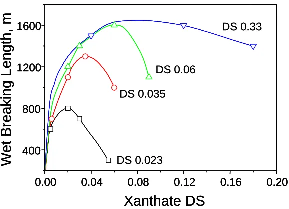
low DS (DS of 0.023, 0.035, and 0.06) but was about 2 to 3 for tertiary amines with a high DS of 0.33 (see Figure 1.2). The authors also found that polyampholytes with quaternary amines

substitution were slightly more effective than those with tertiary amines.

More recently fully synthetic polyampholytes were systematically introduced to enhance paper strength by our labs 9, 22-27. The employed polyampholytes were prepared by free-radical

polymerization of cationic monomer N-[3-(N’,N’-dimethylamino)propyl]acrylamide (DMAPAA), a tertiary amine, anionic monomer methylene butanedioic acid (known as itaconic acid, IA) and

neutral acrylamide (AM) monomer. The advantages of synthetic polyampholytes over natural-based ones include the higher charge density that can be achieved; simple control of the molecular weight and charge ratio of cationic and anionic groups; uniform molecular weight

(23)

used here (see Figure 1.3). Under the experimental conditions used, polyampholytes were applied

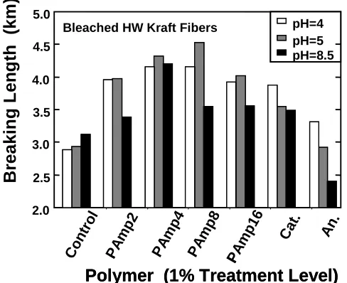
at 1% addition level on bleached hardwood kraft fibers. Paper’s breaking length increased 20-50% compared with control experiments. An interesting phenomenon reported was that the strength increased with the charge density and reached the maximum for polyampholytes of intermediate

charge density (PAmp4 and PAmp8, see Chapter 3 from detailed nomenclature) and then the strength fell with highly charged polyampholytes. A near neutral pH was found to be optimum

condition for strength performance. This could be explained by the fact that under this condition, which is close to the iso-electric point (IEP) of the polyampholytes, a maximum efficiency for adsorption is achieved and bonding between fibers is promoted.

0.00 0.04 0.08 0.12 0.16 0.20 400 800 1200 1600

Wet B

reaking Length,

m

Xanthate DS

DS 0.33 DS 0.06 DS 0.035 DS 0.023

0.00 0.04 0.08 0.12 0.16 0.20 400 800 1200 1600

Wet B

reaking Length,

m

Xanthate DS

0.00 0.04 0.08 0.12 0.16 0.20 400 800 1200 1600

Wet B

reaking Length,

m

Xanthate DS

DS 0.33 DS 0.06 DS 0.035 DS 0.023

Figure 1.2. Wet strength of paper treated with xanthated starch amine (XSA) having various tertiary amine and xanthate degrees of substitution (DS). The paper samples were prepared from unbleached kraft furnish treated with 3% XSA, oven dry pulp basis, at pH 7.0. Figure redrawn from reference 32.

(24)

pitch or stickies and pigments are fixed to the long fibers and fiber fines and, finally, in process

water clarification to settle or float the solids from the white water for solids removal 26, 32, 33. Despite the fact that a number of theoretical and computational efforts has been reported 13, 14, 17, 18, 21, 28, 34-36

, there is a lack of experimental data to advanced our knowledge in this field. The

previous account and ensuing citations is only an example of some of the few reports available in this area. Therefore there is a need for understanding the adsorption phenomena, especially in the

case of polyampholytes, that will lead to new functional additives and improved performance.

2.0 2.5 3.0 3.5 4.0 4.5 5.0 PA mp 2 pH=5 pH=8.5 pH=4

Polymer (1% Treatment Level)

B re a k ing Le n g th ( k m)

Bleached HW Kraft Fibers

PA mp 4 PA mp 8 PA mp 16 Ca t. An . Co ntr ol 2.0 2.5 3.0 3.5 4.0 4.5 5.0 PA mp 2 pH=5 pH=8.5 pH=4

Polymer (1% Treatment Level)

B re a k ing Le n g th ( k m)

Bleached HW Kraft Fibers

PA mp 4 PA mp 8 PA mp 16 Ca t. An . Co ntr ol

Figure 1.3. Effect of macromolecular composition and pH on the tensile strength of polymer-treated bleached kraft fibers at 1000 µS/cm conductivity 25. Structures of polymers denoted as “PAmp 2, 4, 8, 16”, “Cat” and “An” can be seen with more detail in Chapter 3).

In this study we carried out adsorption experiments with a series of polyampholytes having

increased total charge densities at a constant ratio of cationic to anionic monomeric groups and molecular mass. The principal aim of our efforts in polyampholyte research (Chapter 5) is to

(25)

conformation of the respective adsorbed layers.

LUBRICATION AND TRIBOLOGY IN TEXTILE PROCESSING

The science of friction, lubrication and wear, also called tribology, has long been of both

technical and practical interest, since the functioning of many mechanical systems depends on these phenomena 37. This field has received increased attention as the incommensurable waste of

resources resulting from unwanted high friction and wear has become evident. In fact, according to some estimations, proper attention to tribology could lead to economic savings of 1.3% to 1.6% of the Gross National Product (GNP) 38.

In textile processing, fibers, threads and yarns go through many different stages, including pretreatment, dyeing, printing and finishing until they are weaved into end products. Machinery

and equipment are inevitably involved in handling fibers at high shear rates. Fiber materials are subjected to destructive abrasive forces that can be the result of both mutual abrasion between strands and/or between the strands and equipment surfaces. In order to control friction and reduce

wear between fibers and between fibers and metal surfaces (and other materials such as ceramics, etc.), the use of lubricants is indicated. Fiber lubricants are commonly used during the production

of many different fiber grades, including fiberglass and synthetic fibers such as polyesters, polyolefins, polyacrylics, polyamides, etc.39. A myriad of different lubricant formulations exists depending on the intended use and operation conditions. We worked closely with industry to

identify model fiber lubricant systems. An advisory team provided us with input and shared their industrial expertise. Four general classes of boundary lubricants for low energy polymer surfaces

(26)

(1) High molecular weight, water dispersible products - significantly reduce abrasion

damage to fibers in aggressive textile processes and seem to function most effectively in dynamic, higher speed situations;

(2) Waxy materials - traditional boundary lubricants that function in both low speed (fiber

to fiber) and high speed (fiber to metal, fiber to ceramic) applications;

(3) Low molecular weight polymers that have high affinity for the polymer surface and

tend to structure themselves on the surface and,

(4) Silicone based materials - tend to have high affinity for the surface of many of the polymers that are used in fibers.

Our focus in this research involved nonionic surface-active polymers and silicone surfactants. With the technological development in fiber processing, there is a major trend in

textile operation towards higher speed, higher productivity and better quality. Therefore, the motivation of our research rested on the need to develop better quality lubricants to meet the requirements of fiber processing. This prompted us to understand the structure-property relations

of lubricants that would eventually lead to the design of systems that better meet textile demands.

Lubrication phenomena

Lubrication phenomena are involved when substances such as grease or oil (so-called lubricants) are applied to moving objects to reduce friction. Amonton's law, one of the best known

theories concerning lubrication and friction, was proposed in the 17th century in order to describe sliding friction analytically, at the macroscopic scale 37:

(27)

where μis the coefficient of friction, which is a dimensionless scalar value that describes

the ratio of the force of friction between two bodies, Ff,and the force pressing them together and

the normal force applied, N. From a macroscopic view, μ is a constant, which is related to the

nature of both contacting objects; here the frictional force (Ff ) is independent of the apparent

contact surface. This equation can be applied in many cases, at the macroscopic scale and for sliding objects directly in contact. However, simple experimental observation shows that frictional

forces do depend on the contact area, the surface roughness as well as the chemical nature of the sliding substances.

When dealing with fluid lubricants, it is found that the situation becomes even more

complicated since the gap between the two moving objects may vary. The friction coefficient may depend on the gap between the sliding surfaces as well as the sliding speeds or shear rates.

According to Hamrock 40, four different regimes of fluid film lubrication can be defined, i.e., boundary, mixed, elasto-hydrodynamic and hydrodynamic regimes, depending on the film parameter Λ. A profile of friction coefficient as a function of Λ is illustrated by the Stribeck curve (Figure 1.4). The film parameter, Λ, represents the minimum film thickness separating the two

surfaces and can be quantified by using Equation 1.2:

/ b

V η P

Λ = × (Equation 1.2)

where V is the threadline speed in the case of textile processing; ηb is the bulk viscosity of the

(28)

Frict

ion C

oeff

ici

ent

Film Parameter,

Λ

Boundary lubrication Mixed lubrication Elastohydrodynamic lubrication (EHL) Hydrodynamic lubrication a b Frict ion C oeff ici ent

Film Parameter,

Λ

Boundary lubrication Mixed lubrication Elastohydrodynamic lubrication (EHL) Hydrodynamic lubrication a b

Figure 1.4. Stribeck curve, displaying the different regimes of lubrication. Figure Redrawn from original source of Stribeck curve 40.

In full-film lubrication (i.e. the so-called hydrodynamic lubrication), the surfaces are separated by a thick lubricant film. Ideally, there is no wear of the solid surfaces, and the friction is determined by the rheology, surface chemistry, and intermolecular forces of the lubricant. In

boundary lubrication the performance essentially depends on the boundary film since in this boundary regime the load is carried by the surface asperities and the lubricant film. In the

intermediate, mixed region both the bulk lubricant and the boundary film play key roles. Therefore under these conditions the properties of the adsorbed components of the lubricant, and the chemistry and dynamics of the interfacial region between the tribosurfaces are of utmost

importance.

In the Stribeck curve, the bulk viscosity ηb applies to all the cases considered, from wide to

narrow gaps between the sliding surfaces. However, in reality, the local or microscopic effective

(29)

confined systems of ultra narrow gaps 41. Discontinuous transitions between different dynamic

states (e.g. solid-to-solid or static-to-kinetic sliding transitions) not considered in the Stribeck theory often occur in thin films (produced by the lubricant molecules specifically adsorbed on the surfaces). In addition, the ordering and frictional behaviors of the confined molecules are found to

switch at some critical load, velocity or temperature (which is different from the melting point of the bulk fluid). Therefore, Luengo, Israelahvili and Granick 42 proposed a set of improved

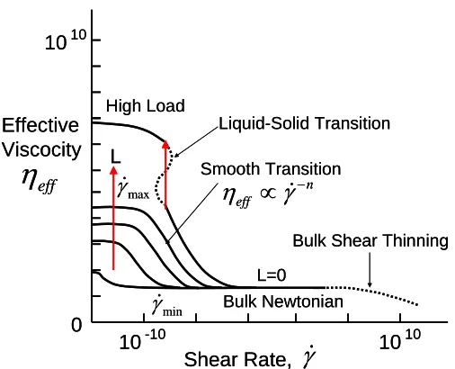
Stribeck-type curves that are based on experimental data typical in engineering conditions. They used three individual figures, shown as Figure 1.5, 1.6 and 1.7, to illustrate how friction changes against with shear rate, sliding velocity and load. In Figure 1.5, three main classes of fluid

behaviors can be distinguished: (1) Thick film, elastro-hydrodynamic sliding: At zero load (L=0), ηeff is independent of the shear rate except that shear–thinning may be displayed when shear rate is

sufficiently large. (2) Boundary layer film, intermediate regime: A Newtonian regime is observed at low loads and low shear rates, but ηeff is much higher that the bulk value, ηb. As the shear rate

increases beyond γ_min, these systems reach a point where the effective viscosity starts to drop with

a power-law dependence on the shear rate. As the shear rate increase still more, beyond γmax, a second Newtonian plateau is again encountered. (3) Boundary layer films, high load: The ηeff

continues to grow with load and the behavior is Newtonian provided that the shear rate is

(30)

0

10-10 1010 1010

L

High Load

Liquid-Solid Transition Smooth Transition

Shear Rate,

γ

Bulk Shear Thinning

min

γ Bulk Newtonian

L=0 Effective Viscocity eff

η

n eff

η

∝

γ

− max γ 0

10-10 1010 1010

L

High Load

Liquid-Solid Transition Smooth Transition

Shear Rate,

γ

Bulk Shear Thinning

min

γ Bulk Newtonian

L=0 Effective Viscocity eff

η

n eff

η

∝

γ

− max γ

Figure 1.5. Proposed generalized friction map of effective viscosity plotted against shear rate. Figure redrawn from reference 42.

The corresponding generalized map of friction force plotted against sliding velocity in

various tribological regimes is shown in Figure 1.6. In this figure, with increasing load, the Newtonian flow in the elasto-hydrodynamic (EHD) regimes crosses into the boundary regime of

lubrication. Note that at the highest velocities, even elastrohydrodynamic (EHD) lubrication lowers the shear stress response. At the highest loads (L) and smallest film thickness (D), the friction force passes through a maximum (the static friction, Fs), followed by a regime where the

friction coefficient (µ) is roughly constant with increasing velocity (i.e. the kinetic friction, Fk, is roughly constant). Non-Newtonian shear-thinning is observed at somewhat smaller load and larger film thickness; the friction force passes through a maximum at the point where De~1 (De, the

Deborah number, is the point at which the applied shear rate exceeds the natural relaxation time of the boundary layer film). The velocity axis from 10-10 to 1010 (arbitrary units) indicates a large span.

(31)

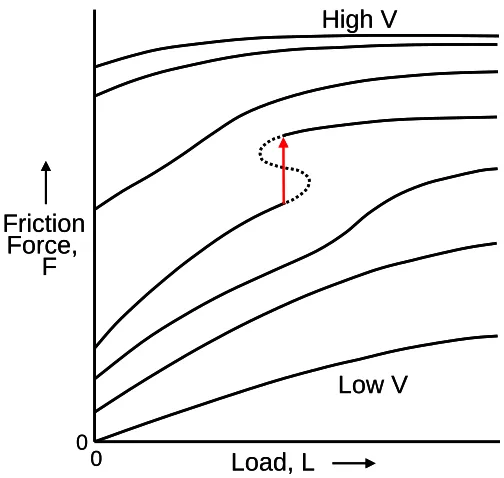
first moderately, then more rapidly, with increasing V. A discontinuous transition to F independent

of L is eventually expected.

Boundary Regime

EHD Regime

Liquid-like bulk (L=0, D=∞) Newbonian Flow High L Small D Solid-like (creeep) Stick-Slip Regime Plastic Flow μ≈constant Fk Fs Amorphous 1 De≈ 1 eff η _∝γ− Friction Force,F effVA F D η =

Sliding Velocity, V

10-10 1010

1010

1

Fk

Boundary Regime

EHD Regime

Liquid-like bulk (L=0, D=∞) Newbonian Flow High L Small D Solid-like (creeep) Stick-Slip Regime Plastic Flow μ≈constant Fk Fs Amorphous 1 De≈ 1 eff η _∝γ− Friction Force,F effVA F D η =

Sliding Velocity, V

10-10 1010

1010

1

Fk

Figure 1.6. Proposed generalized friction map friction force plotted against sliding velocity. Figure redrawn from reference 42.

Friction curves illustrate the phenomena and trends on how friction or friction coefficient varies with operational parameters at a macroscopic scale. However, several issues are still unexplained, for example, what is the origin of friction and why does friction change in the fashion

presented in these figures? To answer these questions we have to resort to studies at the nano or molecular levels. This is the so called molecular tribology, which focuses on the lubricant films’

(32)

Friction

Load, L

Low V High V

F Force,

0 0

Friction

Load, L

Low V High V

F Force,

0 0

Figure 1.7. Proposed generalized friction map of friction force plotted against load. Figure redrawn from reference 42.

While this thesis covers the general topic of boundary lubrication, only a few parameters

were studied. Our focus lay in the chemistry and adsorbed layer state of nonionic and silicone surfactants. Issues related to roughness, asperities and others are not considered here.

Thin film lubrication

Lubrication in textile processing

Within the boundary lubrication regime, the load is carried by the lubricant thin film. A typical lubricant film is very thin, usually 100 nm or lower, i.e., only several to hundreds of molecules thick 43-45. Studying the structure of lubricant thin films and how the molecules organize

(33)

intended to be retained onto the surface of the fibers, specially if the lubricant on fiber surfaces

would interfere with successive processes, such as finishing and dyeing. However, the robustness or strength of adsorbed layer in textile processing is an issue that hasn’t been addressed systematically.

Property changes and transitions in thin films

The properties of lubricant thin films change depending on their distance from the surface.

When the thickness of the adsorbed film is comparable to the dimensions of the lubricant

molecules themselves, the properties of the thin film is quite different than that of the bulk medium 41

. As shown in Figure 1.8, the effective viscosity, elasticity and relaxation time grow with

diminishing thickness and diverges when the film thickness is sufficiently small. In this case, classical continuum considerations, which apply to the bulk phase, do not apply to thin films.

•Viscosity

•Elasticity

•Relaxation

time

Solid Boundary

liquid

Bulk liquid

Continuum properties

Å

nm

μ

m

•Viscosity

•Elasticity

•Relaxation

time

Solid Boundary

liquid

Bulk liquid

Continuum properties

Å

nm

μ

m

Figure 1.8. Schematic diagram of how the effective viscosity, elasticity and relaxation change with thickness of a lubricant film. Figure redrawn from reference 41.

(34)

decreases exponentially from the edges towards the center in systems under Hertzian contact.

Hertzian contact is an ideal model to describe deformation and lubrication. In this model, only small deformation occurs in contact areas, contacting bodies are elastic and therefore only vertical forces are considered. Granick et al. 47, 48 studied the influence of shear behavior on polymer

interfacial diffusion. According to their results, shear did not modify substantially the Brownian diffusion.

Phase behaviors of lubricants may change in confinement conditions. This may be one of the reasons why properties of thin films differ from the bulk. Confinement-induced phase states of lubricant layers could change from liquid-like to an amorphous state and then to a solid-like state 49.

Low friction is exhibited by solid-like and liquid-like layers; high friction is exhibited by

amorphous layers. A change of some factors, such as temperature and humidity generally can shift

the phase status from the solid-like towards the amorphous or liquid-like states.

Confinement-induced solidity of lubricant was observed by Denirel and Granick 50 by placing octamethyl cyclotetrasiloxane (OMCTS) liquids between two rigid mica plates when spacing was

decreased below ca. 10 molecular dimensions. This phenomena was also observed by Israelachvili and coworkers 51, 52 by shearing polybutadiene (PBD) of 7000 molecular weight . They found that

at low shear rates, PBD exhibited bulk-like properties in films thicker than about 200 nm. In thinner films (200-20 nm), the shear viscosity ηeff and moduli G' and G'' became quite different

from those of the bulk. On entering the tribology regime (film thickness <30 nm) PBD exhibited

highly nonlinear behavior and yield points, indicative of phase transitions to "glassy" or

(35)

solid-like phase of the liquids under progressive confinement take place abruptly at a distance

around six molecular layers. The films that are thinner than six molecular layers behaved in a solid-like fashion, in the sense that they required a critical stress in order to shear them.

Structure of lubricant films

Why can lubricants reduce friction, i.e. how do lubricants work and how do the lubricant molecules behave under shear? This question is being investigated by several groups. Lubricant

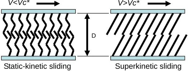
molecules organize themselves under shear as illustrated in Figure 1.9 by Yoshizawa et al 49. A critical velocity Vc* exists; if the sliding velocity of two surfaces are below it, a polymeric lubricant film exhibits amorphous structure and chains of polymer interplay and entangle with

each other. In this case high friction is produced (static-kinetic sliding). This phenomenon supports that chain interdigitation is an important molecular mechanism that gives rise to “boundary”

friction and adhesion hysteresis of monolayer-coated surfaces. If the sliding velocity of two surfaces is above the critical velocity, polymer chains will be aligned or “combed” by shear into an ordered conformation and therefore will result in very low friction (superkinetic sliding).

Figure 1.9. Lubricant molecules organized by shear. Figure redrawn from reference 49

Shear–induced alignment of lubricant molecules was supported by a number of Static-kinetic sliding Superkinetic sliding

D

(36)

experiments. Frantz and co-workers 54 adsorbed polyisoprene onto a single solid surface and found

that the backbone of the polymer oriented in the direction of flow. They also found that the extent of orientation increased with increasing molecular weight. The structure of the lubricant, such as chain length 54, packing densities 55, 56, and nature of the polymer (brush-like 11 or grafted polymer 57

and chain ends 58) influenced its alignment under shear.

Within these investigations, the work of Urbakh et al 57 is very significant. They used

grafted polyelectrolytes, hyaluronan and hylan, to mimic cartilage lubrication. These polysaccharides (outermost cartilage layer) were not expected to be the responsible molecule for the great lubricity of cartilage; however, the authors found that they may contribute to the load

bearing and wear protection in these surfaces. Their study showed that a low coefficient of friction is not a requirement for, or necessarily a measure of, wear protection. This gives us much

inspiration to think about the design and formulation of lubricants and their layer structure for wear protection.

Techniques to study thin films and lubrication phenomena

It is well known that the function of thin films in boundary lubrication and mixed

lubrication regimes is to offer friction reduction and wear protection. Therefore, thin film lubrication is a phenomenon that exists universally in conventional tribological systems. A better understanding of thin film lubrication will improve our knowledge of how lubricants work, and

will result in the development of superior lubricant formulations for use in industry, and also will improve our capabilities to predict tribological failures.

(37)

the expansion in computer power offered an unprecedented opportunity to unveil how lubricant

polymers behave under boundary lubrication conditions (at the atomic/molecular or nano levels). Atomic force microscope (AFM) with lateral force capabilities measures the friction between a substrate and a few to several hundred atoms on a sharp tip. The lateral resolution can be less than

an atomic spacing 59, 60. On the other hand the surface force apparatus (SFA) can measure the forces between atomically flat surfaces as their separation is varied with Ångstrom level resolution.

The friction and adhesion can be studied as a function of the chemistry and thickness of the material between the surfaces 11, 61-65. Computer simulation has played an important role in interpreting and explaining the findings from these experimental methods. Computer simulations

and theoretical investigations have shed much light on the molecular details underlying both structural and dynamic behavior of liquids in the highly confined regime 66, 67.

From the molecular view, lubrication molecules adsorb on a metal or organic surface with ordered or oriented chains. As mentioned before, the interactions of solid surfaces and lubricant films could be physical adsorption, or chemical reactions 68. The thickness or the adsorption mass

and structure of the adsorbed layer are crucial to the performance of lubrication 69-72. SPR and QCM both are well-established noninvasive techniques capable of providing a wealth of

information about interfacial phenomena in situ, in real time and in fluid media 3, 8, 73-87. The resolution of surface plasmon resonance (SPR) and quartz crystal microbalance (QCM) are in the Ångstrom/nano scale. Even though friction cannot actually be measured with QCM and SPR, they

(38)

adsorbed layers 88. The advantages of QCM are that it can provide some intrinsic properties of the

adsorbed film, such as its viscoelasticity (QCM with dissipation monitoring) and coupled water (if results from the QCM are compared with those from SPR or ellipsometry).

The ability to evaluate dynamic behaviors is quite similar with both systems from a

technical point of view, but when it comes to sensitivity they differ. Table 1.1 compares the QCM-D and SPR techniques. QCM-D systems are more sensitive to water-rich and extended

layers, while the SPR system is favored for compact and dense layers. The reason to this difference is due to the different physical principles by which the coupled mass is measured. The mass-uptake estimated from SPR data is based on the difference in refractive index between the adsorbed

materials and water displaced upon adsorption. Therefore, water associated with the adsorbed materials, e.g. the hydration water, is essentially not included in the mass determination. In

contrast, changes in frequency acquired with QCM-D are affected by the coupled water arising from hydration, the viscous drag and/or entrapment in cavities in the adsorbed film. This means that the SPR response is proportional to the "dry mass", while in QCM-D measurements the layer

is essentially sensed as "hydrogel" composed of the macromolecules and coupled water. While SPR measures one parameter only, the additional information contained in energy dissipation

measurements when using QCM-D increases the base for a detailed interpretation. Changes in the dissipation are related to the shear viscous losses induced by the adsorbed layers, and thus provide information that has the potential to identify structural differences between different adsorbed

(39)

To reveal the intricacies of boundary lubrication, techniques to probe adsorption, friction,

topography accompanied by molecular dynamics simulation, were used in our lab. In this chapter, we discuss the principles of SPR and QCM and their applications to boundary lubrication. In the next sections and also in Chapter 6 to 8, we focus our attention in the measurement of adsorption of

lubricants in textile processing by SPR and QCM. Finally, we will also introduce briefly the measurement of friction via lateral force microscopy (LMF) and molecular dynamic simulation

(MDS), last chapter of this thesis.

Table 1.1. Comparison between QCM and SPR techniques (*)

Instrument QCM-D SPR

Principles Piezoelectic/electromechnical Optical Resolution 3 ng/cm2 (QCM-E4) in water 10 ng/cm2 in water

Limitation N/A Small molecules with Mw<1000 give very small response

Detection range

The detection range varies from nanometers to

micrometers, depending on the viscoelasticity of the adsorbed film. In pure water it is approximately 250 nm.

~300 nm

Information provided

-Adsorbed mass -Adsorption kinetics -Dissipation

-Total adsorbed mass -Adsorption kinetics

-Reflective index adjacent to metal surface

(*) Source: QCM and SPR manuals and manufacturer websites.

Methods used in this research

Principles or SPR and QCM

Surface Plasmon Resonance (SPR)

A surface plasmon is a charge density wave occurring at the interface between a metal

(40)

the photon electrical field is just right so that it can interact with the free electron constellations in

the gold surface. The photon energy is then transferred to the charge density wave. This phenomenon can be observed as a sharp dip in the reflected light intensity. The angle where the sharp dip happens is called “SPR angle”. Outside the metal surface there is an evanescent electric

field, which decays exponentially. This evanescent field interacts with the close vicinity of the metal. Changes in the optical properties of this region will therefore make the (SPR) angle shift.

This is the principle basis of SPR. A schematic of SPS is shown in Figure 1.10. .

Figure 1.10. Schematics of surface plasmon resonance, from Ref. 89.

The position of the SPR angle depends on the refractive index of the substance with a

low-refractive index close to the sensing surface. The refractive index near the sensor surface changes because of the binding of polymers to the surface. As a result, the SPR angle will change

(41)

wavelength of the probing laser:

2

( )

( ) (sin )

2 ( )( )

f

m s s m m s

f c

f s f m m s

n

d λ ε ε ε ε ε ε ε θ

π ε ε ε ε ε ε

− − +

= Δ

− − (Equation 1.3)

where df is the thickness of adlayer; n is the solvent refractive index; λ is the wavelength of the

incident laser;εf is the dielectric constant of the film; εs is the dielectric constant of the solvent; εm

is the real part of the dielectric constant of the metal; and θc is the critical resonant angle on the

plasmon resonance curve. So for a given system with known solvent and metal,θc is the only

variable. Equation 1.3 can be simplified as:

d_f = Δk (sinθ_c) (Equation 1.4)

where k is a factor that can be obtained after a calibration. In most case, θc is very small and there is

a linear relationship between the amount of bound material and the shift of the SPR angle 79, 83. SPR response values are usually expressed in resonance units, RU (1 RU = 0.0001°) or refractive index units, RIU (1 RU = 0.001 RIU = 1 μRIU ). For most proteins and polymers, changing of 1

RU is roughly equivalent to a change in concentration of about 1pg/mm2 and changing of 10 μRIU

is roughly equivalent to a change in concentration of about 1 ng/cm2 on the sensor surface. The exact conversion factor between RU and surface concentration depends on properties of the sensor surface and the nature of the molecule responsible for the concentration change.

One limitation of SPR technique is that for those compounds with molecular weights smaller than 100 - 200 Daltons can’t be detected because the change in refractive index for small

(42)

totally. However, both situations are not relevant in most cases and linear relationships hold 90. The

reader is referred to a number of excellent review papers 79, 83 and internet resources 90 that discuss SPR and its principles of operation.

Quartz Crystal Microbalance with Dissipation, QCM-D

A QCM crystal consists of a thin quartz disc sandwiched between a pair of electrodes (cf. Figure 1.11a). Due to the piezoelectric properties of quartz, it is possible to excite the crystal to

oscillation by applying an AC voltage across its electrodes (cf. Figure 1.11b).

Figure 1.11. QCM sensor (a) and schematic principle of QCM

The resonant frequency (f) of the crystal depends on the total oscillating mass, including

water coupled to the resonator. When a thin film is attached to the sensor crystal the frequency decreases. If the film is thin and rigid, no or minimum energy dissipation occurs, the decrease in frequency is proportional to the mass of the film. This is Sauerbrey relation 91:

₂

0 2 0

q qt f q qv f c f

m

nf nf n

ρ Δ ρ Δ _Δ

Δ = − = − = − (Equation 1.5)

C = 17.7 ng Hz-1 cm-2 for a 5 MHz quartz crystal. n = 1,3,5,7 is the overtone number.

Since the change in frequency can be detected very accurately the QCM operates as a very diam. 14mm

Quartz

Gold Electrode

(43)

sensitive balance. The quartz crystal microbalance (QCM) was first used to monitor thin film

deposition in vacuum or gas atmospheres at first. More recently, it was shown that the QCM may be used in the liquid phase, thus the number of applications for the QCM increased dramatically. The Sauerbrey relation was initially developed for adsorption from gas phase, it is now extended to

liquid media where it holds in most cases. In order to describe soft adlayers of polymer adsorbing from liquid media, the dissipation value was introduced. Rodahl et al. 80 extended the use of the

QCM technique and introduced the measurement of the dissipation factor simultaneously with the resonance frequency by switching on and off of the voltage applied onto the quartz. The measured change in dissipation is due to changes in the coupling between the oscillating sensor and the

surroundings. It is affected by any energy dissipating process and thus influenced by the layer viscoelasticity and slip of the adsorbed layer on the surface. The dissipation factor D, is the inverse

of the so-called Q factor and defined by:

1 2

disspated

stored

E D

Q πE

= = (Equation 1.6)

where Edissipated is the energy dissipated during one period of oscillation and Estored is the energy stored in the oscillating system. The resonance frequency is measured when the oscillator is on and when it is turned off the amplitude of oscillation, A, can be determined in it decay as an

exponentially damped sinusoidal function:

A t( )=A e₀ −t/τsin(ω ϕt+ )+c (Equation 1.7)

where τ is the decay time, ω is the angular frequency at resonance, φ is the phase angle and

(44)

1.8.

D 1 f

π τ

= (Equation 1.8)

Combinating Equations 1-5 and 1-8, the dissipation changes can be expressed as Equation 1.9. Dissipation changes not only with the properties of the adsorbed layer but also with the density and

viscosity of the solution 81:

1 2 f f q q D n t f η ρ ρ π

Δ = (Equation 1.9)

Generally, soft adlayers dissipate more energy and thus are of higher dissipation value. From this

point of view, dissipation value is an indicator of the conformation of the adlayers. This is the fundamental basis of QCM-D technique.

A practical QCM-D system records the signals of fundamental frequency (5 MHz) and

overtones (e.g. 15, 25 and 35 MHz and even high frequencies for newly developed systems). Each overtone has its own detecting range in thickness. This enables its abilities to measure non-uniform

adlayer. Theoretical work was done by Voinova and coworkers 92. A general equation was derived to describing the dynamics of two-layer viscoelastic polymer materials of arbitrary thickness deposited on solid (quartz) surfaces in a fluid environment.

2 ₂

3 3

2 2 2

1,2

0 0 3 3

1

2 j

j j j

f h h

h η ω η _{ρ ω} η πρ δ = δ μ ω η ⎧ ⎡ _⎛ _⎞ ⎤⎫ ⎪ _⎢ _⎥⎪ Δ ≈ − _⎨ + − _⎜ _⎟ _⎬ + ⎢ ⎝ ⎠ ⎥ ⎪ _⎣ _⎦⎭⎪ ⎩

∑

(Equation 1.10) 2 3 3

2 2 2

1,2

0 0 3 3

1

2 2

j j

j j j

(45)

where ρ stands for density; h stands for thickness; η stands for viscosity and δ stands for the

viscous penetration depth (δ 2η ρω

= ). The subscript 0, 1, 2 and 3 denote quartz crystal, layer 1,

layer 2 and bulk solution respectively. From this model, the shift of the quartz resonance frequency and the shift of the dissipation factor strongly depend on the viscous loading of the adsorbed layers

and on the shear storage and loss moduli of the overlayers. These results can readily be applied to quartz crystal acoustical measurements of the viscoelasticity of polymers which conserve their shape under the shear deformations and do not flow, and layered structures such as protein films

adsorbed from solution onto the surface of self-assembled monolayers. By measuring at multiple frequencies and applying this model, which has been incorporated in Q-Sense software QTools ™,

the adhering film can be characterized in detail: viscosity, elasticity and correct thickness may be extracted even for soft films when certain assumptions are made.

In summary, QCM technique with dissipation monitoring has the advantage that it can measure the adsorbed amount via Δf and conformation via ΔD, simultaneously in situ and in real

time. Furthermore, some adlayer properties, such as viscosity, elasticity and effective thickness

can also be extracted from a set of measurements, as will be illustrated later in the respective chapters.

Applications of SPR and QCM to Study Lubricant Films

Monitoring adsorption and desorption of lubricants

(46)

are useful to find out if a lubricant has affinity or not with a given organic/polymeric substrate.

Secondly, they enable elucidation of how strong the affinity is and, thirdly, QCM and SPR can measure the actual kinetics of adsorption and desorption.

Typical adsorption curves can be seen in other chapters of this thesis. If we take Figure 8.2

as a reference, it can be succinctly explained here that we compared the affinity difference for a commercial silicone-based lubricant onto polyethylene (PE) and polypropylene (PP) surfaces. The

experiment started with a baseline, and then silicone lubricant solution was injected in the loop. Correspondingly, a sharp frequency drop and dissipation raise were observed (see Figure 8.2) since the lubricant adsorbed on the surface. When both frequency and energy dissipation reached

their equilibrium state, large amount of pure water was injected to rinse. A sharp rise in frequency and a sharp drop in dissipation could then be observed. This behavior indicated that lubricant

molecules in bulk as well as molecules loosely bonded on the surface were removed by rinsing. During the experimental process, the injection speed of the sample was kept constant at 0.1ml/min. Comparing the adsorption curves of PP with those of PE, the frequency change for PP film was

observed to be larger than that for PE film, either on the basis of total adsorption (-22.5 Hz vs -18.4 Hz) or adsorption after rinsing (-10.2 Hz vs -8.6 Hz). This indicates that the affinity of silicone

(47)

Figure 1.12. Time-dependent frequency change of QCM for EM and AF adsorbed on QCM crystal at 200 °C. From reference 93.

Lubricant degradation can also be measured by the QCM technique. In order to monitor the

degrading process of lubricants at high temperature, Wang et al. 93 developed a QCM system which could endure high temperatures (more than 200 ºC). They evaluated the thermal stability of polyol ester lubricants in the QCM chamber. Figure 1.12 provides an example that demonstrates

how different lubricants showed different sensitivities to temperature. Here the lubricants were hold in a T-controlled chamber. The lubricants degraded gradually when they were heated to very

high temperature leaving solid residues on the tested QCM crystal surfaces. Two commercial-grade pentaerythritol tetrapelargonate based lubricants, EM, AF (codes for two commercial lubricant compositions), are shown in this figure. During the first nine hours, both EM

and AF didn’t change too much with the temperature treatment which indicated that both lubricants were stable. However, after exposure to high temperatures for nine hours the frequency

(48)

than AF at the tested temperature of 200 ºC. The results from QCM can thus provide an integral

picture of the thermal stability of lubricants from the quantitative, real-time, in situ information it generates during the thermal decomposition of the lubricants.

Kinetics of adsorption and desorption

Figure 1.13. Change in frequency for 5 MHz Si crystals upon injection of OTS (10 mM). The arrow indicates injection time. Insert is an enlargement of the region indicated by the box, to show the stability level. Figures from reference 7.

The time-dependent signals (changes in frequency and refractive index in QCM and SPR,

respectively) can be used to study the adsorption kinetics. The Langmuir isotherm, an often used model, is a simple equation that relates adsorption and concentration. For such a mechanism, the adsorption rate can be written as represented in Equation1.12:

( )t β[1 exp( t)]

φ α

α

= − − (Equation 1.12)

where φis the fraction of free active sites on the surface, α= C k + k_b _af _ar and β= C k_b _af. Cb is the

concentration of lubricant, while kaf and kar represent the constants of adsorption and desorption, respectively. The parameters α and β can be obtained by fitting the frequency to Equation 1.12. An

(49)

between α and Cb, the values of kar and kaf can be determined. The results of the adsorption rate

calculations, the equilibrium constant (K =k /k ), and free energy of adsorption were also _eq _af _ar

determined by Equation 1.13:

Δ = −G RTlnK_eq (Equation 1.13)

Conformation of lubricant films revealed by the QCM-D

As described before, the conformation of adsorbed lubricant layers can be derived from QCM data. For rigid, ultrathin, and evenly distributed adsorbed layers, the Sauerbrey equation 91

describes successfully the proportional relationship between the adsorbed mass (m) and the shift of the QCM crystals’ resonance frequency (f ). Under these conditions, the dissipation value is a constant. It doesn’t change with time or with increased adsorbed mass. On the other hand, if the

adsorbed material exhibits a viscoelastic behavior, such as for layers of proteins, substantial deviations from the Sauerbrey equation can occur. Using ΔD–Δf plots one can eliminate time as an

explicit parameter and as concluded in previous studies 6, 81, 88, 94, the absolute slopes and their changes provide information about the kinetic regimes and conformational changes 88. These slope values indicate the conformation of adsorbed layer: The lower value indicates a softer layer. If

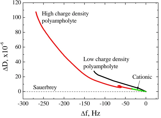
more than one slope exists, it can be concluded that more than one conformation states of the adsorbed layer are present during the adsorption process. Figure 1.14 shows the relation between

dissipation change and frequency change for low and high charge density polyampholytes. From these slope values one can draw meaningful conclusions including the fact that the low charge density polyampholytes tend to form a uniform layer. For high charge density polyampholytes, the

(50)

compared with the outer layer, which exhibits a flat slope.

-300 -250 -200 -150 -100 -50 0

0 20 40 60 80 100 120

Cationic Low charge density

polyampholyte

Δ

D

, x10

-6

Δ

f, Hz

High charge density polyampholyte

Sauerbrey

Figure 1.14. ΔD-Df profiles for polyampholyte adsorption on silica surfaces. The low charge density polyampholite (PAmp4) consisted of 5% cationic and 4% anionic groups while the high charge density pol