Precision geoid determination by spherical FFT
in and around the Korean peninsula
Hong-Sic Yun
Department of Civil Engineering, Sungkyunkwan University, Korea (Received April 3, 1998; Revised September 17, 1998; Accepted October 12, 1998)
This paper deals with the precision geoid determination by a gravimetric solution in and around the Korean peninsula. A number of data files were compiled for this work, containing now more than 69,900 point gravity data on land and ocean areas. The EGM96 global geopotential model to degree 360 was used in order to determine the long wavelength effect of the geoid surface. By applying the remove-restore technique the geoid undulations were determined by combining a geopotential model, mean free-air gravity anomalies and height in a Digital Elevation Model (DEM). Computation involves a spherical approximation to conduct the Stokes’ integration by a two dimensional spherical Fast Fourier Transform (FFT) with 100% zero-padding. A terrain correction was also computed by FFT with a spherical approximation of the Residual Terrain Model (RTM) terrain correction integration. Accuracy estimates are given for absolute geoid undulations using 78 GPS/Leveling stations. The comparative evaluation gives the bias of 0.187 meters and standard deviation of 0.28 meters, respectively. The relative accuracy achieved was of the order of 3.1 ppm for baselines between 10 and 350 kilometers.
1.
Introduction
Successful development of the Global Positioning Sys-tem (GPS) permits the determination of positions very ac-curately in a terrestrial three dimensional Cartesian frame, and theX,Y,Z coordinates obtained are easily convertible into ellipsoidal coordinates—latitude, longitude and height above the ellipsoid. However, the conversion of ellipsoidal height into an orthometric height requires an accurate geoid undulation. The relative accuracy of the gravimetric geoid heights should meet at least the same accuracy level (see, e.g., Schwarzet al., 1987; Li, 1993). This means that by combining relative ellipsoidal heightshfrom GPS and rel-ative geoid heightsN, orthometric height differences can be determined (H =h−N), providedN is of the same accuracy ash. To achieve such accurate results, more advanced methods currently available for gravimetric geoid determination should be used and the different data types should be optimally combined (see, e.g., Tziavos, 1993). GPS highlighted the necessity of an accurate geoid model. Especially in order to meet the needs of geodetic leveling, a geoid of 10 centimeters precision level should be provided.
In Korea, Yun and Adam (1994) evaluated some geopo-tential models to determine the optimal reference field for the geoid solution in the Korean peninsula. A comparison of the solutions with surface gravity data, GPS data and each mod-els in the Korean peninsula showed that the OSU91A (Rapp
et al., 1991) models to degree 360 gives the best fit. Yun (1994) presented a gravimetric geoid solution by fast Fourier Transform technique. Yun (1995) studied the geoid determi-nation by numerical integration, FFT on the plane and on the
Copy right cThe Society of Geomagnetism and Earth, Planetary and Space Sciences (SGEPSS); The Seismological Society of Japan; The Volcanological Society of Japan; The Geodetic Society of Japan; The Japanese Society for Planetary Sciences.
sphere with many options. This study illustrates the com-parison results of geoid undulations derived from different solutions. Leeet al.(1996) improved the Korean geoid re-ferred to OSU91A with joint project of National Geography Institute.
The NASA Goddard Space Flight Center and the Ohio State University (Lemoine et al., 1996) announced the EGM96, an improved degree 360 spherical harmonic model. The EGM96 was improved the data holdings over many of the world’s land areas, including Alaska, Canada, parts of South America and Africa, Southeast Asia, Eastern Europe and the former Soviet Union. In addition to the above surface gravity data acquisitions, there have been major efforts to im-prove the National Imagery and Mapping Agency (NIMA)’s existing 30’ mean anomaly data base through mean anomaly contributions over various countries in Asia (Lemoineet al., 1996). The distribution and extent of the surface gravity data is a major improvement on the data available for the OSU91A. The EGM96 model represents the latest devel-opment in high degree geopotential models which combine satellite data and the available surface and marine gravity data from NIMA.
This study represents an updated version of the Korean geoid using all available data, including the most recent EGM96 model, surface gravity data and digital elevation model. By applying the remove-restore technique, high pre-cision gravimetric geoid undulations were determined by combining the EGM96 model, mean free-air gravity anoma-lies and heights in the DEM. The new gravimetric geoid is based on the Stokes’ integration of gridded gravity data by the multi-band spherical FFT method, using terrain reductions for smoothing the data prior to FFT.
Fig. 1. Difference between gravity anomalies implied by the OSU91A and EGM96 geopotential models, Contour interval: 2 mGal.
2.
The Available Data
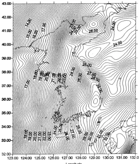
Various geopotential models are available in assessing the contribution of geopotential model on geoid. Yun and Adam (1994) conducted extensive numerical tests on the ability of geopotential model in representing the gravity field in the region encompassing the Korean peninsula. These tests are based on a comparison of the solutions with respect to the sur-face gravity data, GPS data and each models. The EGM96, as the latest version of geopotential model, has become avail-able recently. Figure 1 illustrates the improvement in the new EGM96 model, compared with the OSU91A in the northern area and the ocean area in and around the Korean penin-sula. In the tests with GPS/Leveling, the geoid undulations derived from measurements of benchmarks using 78 GPS height anomalies are compared to the geoid undulations de-rived from EGM96 and OSU91A models. GPS data were obtained from Korea Astronomy Observatory and measured by Sungkyunkwan University. GPS and leveling tests are summarized in Table 1. A comparison between results ob-tained from OSU91A and EGM96 showed that the latter model had a smaller bias in test areas, and for this reason it was chosen as the reference model in all computations. Figure 2 shows the quasi-geoid undulations computed from EGM96 referred to GRS80.
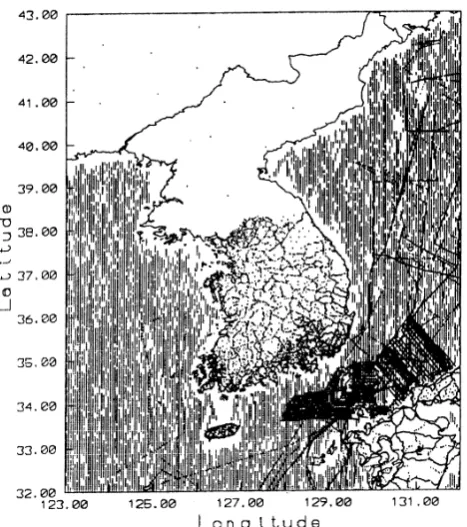
Point gravity data were supplied from the National Geog-raphy Institute (NGI), Prof. Choi, K. S. in Pusan University, and Bureau Gravimetrique International (BGI) as shown in Fig. 3. The data were received in two basic forms: paper and digital listings. Raw data obtained arefiltered to delete duplicate or obviously wrong data. These digital data were reformatted and corrected to the required processing
param-Fig. 2. The quasi-geoid undulations based on the EGM96 geopotential model complete to degree and order 360, Contour interval: 20 cm.
Table 1. Comparison of geopotential and GPS/Leveling height anomalies, in meters.
78 Stations Min. Max. Mean S.T.D.
OSU91A −1.071 1.631 0.420 0.556
EGM96 −0.819 1.469 0.344 0.498
eters and datum used in this study. Gravity anomalies in the ocean area are based on a combination of Geosat, ERS-1 and Topex/Poseidon databases developed at BGI. From the free air gravity anomaly set (69,900 points), a new set of Faye anomalies has been derived by simply adding the terrain cor-rections to the free air anomalies. In Table 2 the statistics of the original free-air gravity anomalies, the gravity anomalies computed from the EGM96, the reduced Faye anomalies and the residual gravity anomalies are presented.
Digital elevation model with grid span of 250 m×250 m on land part of southern area of peninsula is provided by the Korean Energy Resource Institute. In order to compute the terrain correction and their contribution of geoid prediction, a 3×3gridded DEM was generated by means of a minimum curvature spline.
3.
Practical Computation
The well-known Stokes formula for the geoid undulation relative to the reference ellipsoid is
N= R 4πγ
σ
Table 2. Statistics of the gravity anomalies and geoid heights.
Geopotential model Max. Min. Mean RMS S.T.D.
OSU91A N(m) 35.17 10.30 24.19 24.78 5.40
g(mGal) 85.72 −95.14 16.41 24.03 17.55
EGM96 N(m) 33.68 8.18 23.68 24.28 5.38
g(mGal) 107.97 −110.24 18.16 28.04 20.97
Faye anomalies 159.59 −90.12 16.26 21.20 15.38
Residual anomalies 141.21 −68.70 −1.60 18.32 15.15
Fig. 3. Distribution of gravity data in and around the Korean peninsula (69,900 points).
whereS(ψ)is the Stokes’function,Ris the mean radius of the Earth, andσ denotes the Earth’s surface.
By using Eq. (1), the geoid undulation, i.e. the physical
figure of the earth, can be determined from the gravity ob-servation. As we can easily understand from the equation, we need to know the gravity values on the entire surface of the earth for the geoid determination. It is not practical to get gravity data densely throughout the globe. When a global geopotential model is available, Stokes’integral can be modified to integrate gravity anomalies over small capσ (Kuroishi, 1995).
where NGM and gGM are the geoid undulation and the gravity anomaly, respectively, calculated by the geopotential model. The contribution of the geopotential model, NGM
and gGM can be found in many publications (see, e.g., Heiskanen and Moritz, 1967; Kearselyet al., 1985) and will not be illustrated here.
In most of geoid computations, the topographic masses are moved or removed resulting in changes in the geopo-tential. The change in potential give rise to the systematic errors (indirect effect) in computed geoid. The indirect ef-fect on the geoid is given by Grushinsky’s formula (see, e.g., Wichiencharoen, 1982):
Nind=
πGρH2
γ (3)
whereG is the Netwonian gravitational constant, H is the height of the running point,σis the assumed constant density of the topography.
The main problem with the classical Stokes’integration is that it requires that the gravity data should be reduced (or downward continued) to the geoid. Such a reduction requires a knowledge of the density distribution in the topography above the geoid. This can be circumvented in practice by assigning a reasonable constant density to the topographic masses, thus simplifying the formulae and making them more suitable in practical evaluation.
The present gravimetric geoid solution is build up in the usual “remove-restore” technique, yielding in principle quasi-geoid heightsζ.
ζ =ζ1+ζ2+ζ3 (4)
whereζ1 gives the contribution of the geopotential model, while ζ3 gives the contribution of residual gravity anoma-lies(g)with the effect of the geopotential model and the terrain removed. ζ2 gives the indirect effect of the terrain reduction. Terrain effects have been removed in a consistent RTM terrain data reduction, taking into account the topo-graphic irregularities relative to the mean height surface with a resolution of approx. 100 km (see Forsberg, 1985).
Table 3. Statistics of the topographic effects.
DEM effects Max. Min. Mean S.T.D.
1 km×1 km DEM source (m) 1656.37 0 146.16 —
Gravity effect (mGal) Mass line 46.29 0 0.81 1.47
Geoid effect (meter) Mass line 0.15 −0.06 0.00 0.04
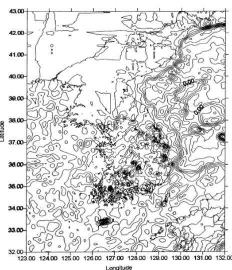
Fig. 4. Residual gravity anomalies from geopotential model minus Faye gravity anomaly, Contour interval: 10 mGal.
whereg1cis thefirst term of the Molodensky series for the reducedfield, which for most practical purposes can be ne-glected. The expression (5) can be written as a spherical convolution in latitude and longitude(φ, λ)for a given ref-erence parallelφref.and by utilization of a number of bands a virtually exact convolution expression may be obtained by a suitable linear combination of bands. For each band the convolution expression can be evaluated by FFT using
Np=g(φ, λ)sinφ⊗Sref.(φ, λ)
=F−1{F(gsinφ)F(Sref.)} (6)
whereSref.is a modified Stokes’kernel function, and⊗is the convolution operator andFandF−1are the two dimen-sional Fourier transform operator and its inverse (Forsberg and Sideris, 1993).
The topographic restore signal(ζ2)is evaluated simultane-ously with Eq. (6) usingfirst-order mass-layer approximation to the RTM geoid effect given in Forsberg (1985). By merg-ing these computations, the data for FFT will actually turn
Table 4. Statistics of the residual geoid undulations computed by spherical FFT applied 100% zero-padding, in meters.
Min. Max. Mean S.T.D.
Residual undulation −4.061 2.116 −0.148 0.394
into a modified Faye anomaly
gFFT=g+2πGρ(h−href.) (7)
and thus be similar to Helmert methods based on Faye anoma-lies, but still in principle the method gives height anomalies
ζ, and the outcome of the computation is the quasi-geoid. Pre-processing of geoid computation involves the com-putation and removal of the geopotential model and terrain contributions from the free-air gravity anomaly. The terrain corrections were computed on a 3×3grid using DEM data in land part of the southern area of the Korean peninsula. In this study the Fortran program TC2DFTPL which can compute the topographic gravimetric correction using two dimensional FFT and uses as mass line topographic model was applied. TC2DFTPL was obtained from Yecai Li of the University of Calgary. Table 3 summarizes the statistics of both the terrain corrections and their contributions in geoid prediction. The results (Table 3) indicates that the standard deviation of the terrain correction by means of the mass line model is 1.47 mGal and the maximum value is 46.29 mGal. The residual gravity anomalies were calculated by simply subtracting the contribution of EGM96 model complete to degree and order 360 from the reduced gravity anomalies. Figure 4 shows the residual gravity anomalies.
The gridded, reduced gravity anomalies have subsequently been converted to geoid undulations by using two dimen-sional multi-band spherical FFT method. The data are grid-ded by minimum curvature spline.
Table 5. Comparison of gravimetric and GPS/Leveling height anomalies, in meters.
Absolute (m) Relative Distance (km)
(m) (ppm)
No. of points 78 78 78 78
Min. −0.397 −1.108 −9.6 12.96
Max. 0.572 0.995 7.6 339.08
Mean 0.187 −0.236 −2.1 137.26
S.T.D. ±0.275 ±0.231 ±3.1 —
Fig. 5. Residual geoid undulation obtained from two dimensional spherical FFT, zero-padding applied, Contour interval: 20 cm.
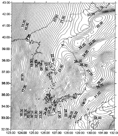
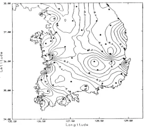
contributions from gravity data and DEM are±0.394 m and ±0.04 m respectively. However, the maximum effects of the gravity data are exceeding 4 meters in the northern area where no data are available. Thefinal geoid undulations were ob-tained by adding three effects. Figure 6 shows thefinal geoid surface referred to the GRS80 ellipsoid. It is noteworthy that the trend of NNE-SSW is recognized in the directions of the topography of the southern land part of the peninsula. Dif-ference of about 14 meters from the NNW to the SSE on land part of the peninsula is apparent.
In order to conduct comparative evaluation, the absolute and relative quasi-geoid are compared with those obtained by 78 GPS height anomalies. The results are summarized in Table 5. Table 5 indicates that the overall agreement between the gravimetric and GPS/Leveling derived height anomalies is about 0.28 meters in terms of standard deviation. Figure 7 shows the locations of GPS stations and the discrepancy
dis-Fig. 6. The resulting geoid map based on the EGM96 geopotential model by means of two dimensional spherical FFT with 100% zero-padding technique, Contour interval: 20 cm.
tribution of between the gravimetric and the GPS/Leveling derived height anomalies. The relative accuracy achieved was of the level of 3.1 ppm for baselines between 12 and 340 kilometers.
4.
Conclusions
Fig. 7. The locations of GPS stations and the discrepancy distributions between the gravimetric and the GPS/Leveling derived height anomalies, Contour interval: 10 cm.
sense and the level of 3.1 ppm or better in relative sense. The differences range about 2 meters in relative sense and less than 1 meter in absolute differences. The resulting geoid shows that the difference from the north-west to the south-east is about 14 meters across the Korean peninsula.
Compared to the existing geoid model of Leeet al.(1996), it is obviously shown that there is a 12 centimeter improve-ment in standard deviation of differences. There are two pri-mary improvement sources. Thefirst is from the improved potential coefficients as shown in Table 1 and the second is the GPS/Leveling data. GPS/Leveling with respect to the Bench marks in present study is expected to enhance the accuracy compared with the one with respect to the triangu-lation points employed in the existing solutions.
References
Forsberg, R., Gravityfield terrain effect computations by FFT,Bull. Geod.,
59, 342–360, 1985.
Forsberg, R. and M. G. Sideris, Geoid computation by the multi-band spher-ical FFT approach,Manuscr. Geod.,18, 82–90, 1993.
Heiskanen, W. A. and H. Moritz,Physical Geodesy, 364pp., Freeman and Company, San Francisco, 1967.
Kearsely, A. H. W., M. G. Sideris, J. Krynski, R. Forsberg, and K. P. Schwarz, White sands revisited-A comparison of techniques to predict deflections of the vertical, UCSE Report No. 20007, Calgary, Alberta, Canada, 1985. Kuroishi, Y., Precise gravimetric determination of geoid in the vicinity of
Japan,Bull. GSI,41, 9–11, 1995.
Lee, S. B., H. S. Yun, and J. H. Choi, Gravimetric geoid determination by Fast Fourier Transform in and around Korean peninsula,J. Korean Soc.
Geod., Photogramm. Cartogr.,14, No. 1, 49–58, 1996.
Lemoine, F. G., D. E. Smith, L. Kunz, R. Smith, E. C. Pavilis, N. K. Pavilis, S. M. Klosko, D. S. Chinn, M. H. Torrence, R. G. Williamson, C. M. Cox, K. E. Rachlin, Y. M. Ming, S. C. Kenyon, R. Salman, R. Trimmer, R. H. Rapp, and R. S. Nerem, The development of the NASA GSFC and NIMA joint geopotential model, Gravity, Geoid and Marine Geodesy, International Symposium, No. 117, 461–469, 1996.
Li, Y. C., Optimized spectral geoid determination, UCGE Report No. 20050, Dept. of Geomatics Engineering, University of Calgary, Canada, 1993. Rapp, R. H., T. H. Wang, and N. K. Pavlis, The Ohio State 1991 geopotential
and sea surface topography harmonic coefficient models, Report No. 410, Dept. of Geodetic Science and Surveying, Ohio State University, 1991. Schwarz, K. P., M. G. Sideris, and R. Forsberg, Orthometric heights without
leveling,J. Surv. Eng.,113, No. 1, 28–40, 1987.
Strang van Hees, Stokes’formula using fast Fourier techniques,Manuscr. Geod.,15, 235–239, 1990.
Tziavos, I. A., Numerical considerations of FFT methods in gravityfield modeling, Nr. 188, Hannover, 1993.
Yun, H. S., Determination of Gravimetric Geoid Solution in South Korea, Gravity and Geoid, International Association of Geodesy, Symposia. 113, IUGG and IAG, Springer, Berlin, 1994.
Yun, H. S., Results of the geoid computation for Korean peninsula, Ph.D. dissertation, Technical University of Budapest, Hungary, 1995. Yun, H. S. and J. Adam, On the global geopotential models in the region of
the Korean peninsula,J. Korean Soc. Geod., Photogramm. Cartogr.,13, No. 1, 95–106, 1994.
Wichiencharoen, C., The indirect effects on the computation of geoid undu-lations, Report No. 336, Dept. of Geodetic Science and Surveying, Ohio State University, 1982.