IJEDR1604124 International Journal of Engineering Development and Research (www.ijedr.org) 834
Abstract—
Hyperspectral imaging could be used to simultaneously obtain large amounts of spatial and spectral information on the objects being studied. This paper provides a comprehensive review on the recent development of hyperspectral imaging applications in food and food products. The potential and future work of hyperspectral imaging for food quality and safety control is also discussed First,focusing on evaluating the model coefficients and convolutionintegral, which are key elements in reducing the predictionerror of the GM(1,N), we replace the existing (composite)trapezoidal rule with (composite) Simpson rule. Bidimensional empirical mode decomposition
(BEMD) has been one of the core activities in image processing .due to its fully data-driven and self-adaptive nature. Hyperspectral imaging which combines imaging and spectroscopic technology is rapidly gaining ground as a non-destructive, real-time detection tool for food quality and safety assessment.
Keywords— Bidimensional empirical mode decomposition (BEMD), classification, genetic algorithm (GA), hyperspectral image, multivariate gray model (MGM), support vector machine (SVM).
I. INTRODUCTION
Over the last few decades, the bidimensional empirical mode decomposition (BEMD) has been developed
as a valuable tool for image processing (e.g., feature extraction). Compared with the previous image analysis techniques, such as Fourier transform or wavelet analysis, the BEMD is empirical, intuitive, and adaptive.s required more human intervention and time consume.
Theoretically, Sharpley and Vatchev provided an alternate characterization of the intrinsic mode functions (IMFs) motivated by the ordinary differential equations (ODEs). Liu and Peng proposed the directional empirical mode decomposition (DEMD), which takes directional quality into account and extracts four features for each pixel in the decomposition. A noiseassisted method referred to as
multidimensional ensemble empirical mode decomposition (MEEMD) was introduced by Wu et al. which bypasses major obstacles of the empirical mode decomposition (EMD) such as the scale mixing. Recently, Xu et al. discussed how the BEMD behaves in aspect of the sampling period, cross-angle, amplitude ratio, and frequency ratio of two components, whereas Kim et al. investigated the smoothing procedure instead of the interpolation and proposed a bidimensional statistical empirical mode decomposition, namely, BSEMD. On the other hand, since its introduction, the BEMD and its variants have found substantial application in science and engineering. For instance, Nunes firstly extended the EMD to 2-D-data scenario. They applied radial basis function (RBF) to obtain envelopes and replaced the Hilbert transform with Riesz transform to study the local properties of the BEMD. Both the triangle-based cubic spline interpolation and thin-plate spline interpolation. The bidimensional empirical mode decomposition (BEMD) has been developed as a valuable tool for image processing (e.g., feature extraction). Compared with the previous image analysis techniques, such as Fourier transform or wavelet analysis, the BEMD is empirical, intuitive, and adaptive. In fact, the decomposition is designed to adaptively extract the bidimensional intrinsic mode. The general aim of this thesis is to further develop methods for accurate classification of hyperspectral data using both the spectral and the spatial information. The focus of the thesis is the incorporation of spatial contextual information into the classification procedure. This raises two principal questions: How to define spatial structures, or neighborhoods for each pixel in the image automatically? Howto combine spectral and spatial information in classification? In the following, we will review the necessary background material for classification of hyperspectral images. Then, we will precise the objectives of this thesis work.
Hyperspectral Image Classification for Based
BEMD Multivariate Gray Module
Mr.Phatangare B.G Prof.Manojkumar
M.E,VLSI and Embedded System M.Tech.,Phd
Dept.Of Electronics and Telecommunication Dept.Of Electronics and Telecommunication
Sahyadri Valley College of Enggineering Sahyadri Valley College of Enggineering
IJEDR1604124 International Journal of Engineering Development and Research (www.ijedr.org) 835 II. BASICCONCEPTOFHYPERSPECTRALIMAGE
A. Basic Block Diagram
The bidimensional empirical mode decomposition (BEMD) has been developed as a valuable tool for image processing (e.g., feature extraction). Compared with the previous image analysis techniques, such as Fourier transform or wavelet analysis, the BEMD is empirical, intuitive, and adaptive. In fact, the decomposition is designed to adaptively extract the bi-dimensional intrinsic mode.
Figure 1: Basic Block Diagram.
The BIMFs with different oscillations from the given image. To date, the development of BEMD can be roughly divided into two aspects: theory and application. Theoretically, Sharply and Vatchev provided an alternate characterization of the intrinsic mode functions IMFs motivated by the ordinary differential equations. Liu and Peng proposed the directional empirical mode decomposition which takes directional quality into account and extracts four features for each pixel in the decomposition. A noise assisted method referred to as multidimensional ensemble empirical mode decomposition was introduced by which bypasses major obstacles of the empirical mode decomposition (EMD) such as the scale mixing.Recently, discussed how the BEMD behaves in aspect of the sampling period, cross-angle, amplitude ratio, and frequency ratio of two components, whereas Kim et al. investigated the smoothing procedure instead of the interpolation and proposed a bidimensional statistical empirical mode decomposition, namely, BSEMD. Moreover, as stated in there are other versions of BEMD that mainly focus on the fast algorithms.
B. Basic Concept of Hyperspectral Image Classification The concept of hyperspectral imaging, also known as imaging spectroscopy, originated in the 1980’s, when A. F. H. Goetz and his colleagues at NASA’s Jet Propulsion Laboratory began a revolution in remote sensing by developing new
optical instruments such as the Airborne Visible/Infrared Imaging
Spectrometer (AVIRIS).
Figure:2 Basic Concept of Hyperspectral Image Classification Thus, hyperspectral imaging is concerned with the measurement, processing and analysis of spectra acquired from a given scene at a short, medium or long distance by typically an airborne or satellite sensor. Examples of hyperspectral airborne imaging systems are AVIRIS. Figure 2: illustrates the hyperspectral imaging concept. As can be seen from the figure, every pixel can be represented as a high-dimensional vector across the wavelength dimension containing the sampled spectrum. Since different substances exhibit different spectral signatures, hyperspectral imaging is a well-suited technology for numerous remote sensing applications including accurate image classification. Hyperspectral image classification, which can be defined as identification of objects in a scene captured by a hyperspectral imaging sensor, is an important task in many application domains.
1) BEMD:
we demonstrate an overview of the BEMD for image processing, the SVM for hyperspectral classification as well as the GA for optimal parameters selection in the k-NN
and SVM. The major merit of the BEMD is that it can represent the given image as an expansion of BIMFs with well-defined in stantaneous frequency. The detailed description of the BEMD can be found in the previous studies Here, we sketch the principle of the BEMD algorithm as follows. To decompose an image s(x, y) ∈ l2(R2), (x, y ∈ N+), the BEMD is implemented through the following sifting
process. Interpolate the local maxima of
s
(
x, y
) to
form an envelope.
IJEDR1604124 International Journal of Engineering Development and Research (www.ijedr.org) 836 Algorithm 1. It is worth noting that by means of the BEMD,
the original image s(x, y) can be represented as s(x, y) = _Q q=1 cq(x, y)+rQ(x, y), where cq(x, y) is the qth BIMF, and rQ(x, y) is the final residue. Each BIMF cq(x, y), q = 1, 2, . . . ,Q significantly represents inherent features of the image s(x, y) and contains an oscillatory mode at different (narrow) range of frequencies. As a result, it is valuable to take these BIMFs as features of hyperspectral images. the development of BEMD can be roughly divided into two aspects: theory and application. Theoretically, Sharpley and Vatchev [1] provided an alternate characterization of the intrinsic mode functions (IMFs) motivated by the ordinary differential equations (ODEs). Liu and Peng proposed the directional empirical mode decomposition (DEMD), which takes directional quality into account and extracts four features for each pixel in the decomposition. A noiseassisted method referred to as multidimensional ensemble empirical mode decomposition (MEEMD) was introduced by Wu et al. [3] which bypasses major obstacles of the empirical mode. decomposition EMD such as the scale mixing. Recently, Xu et al. Discussed how behaves in aspect of the sampling period, cross-angle, amplitude ratio, and frequency ratio of two components, whereas Kim et al. investigated the smoothing procedure instead of the interpolation and proposed a bidimensional statistical empirical mode decomposition , namely, BSEMD. Moreover, as stated in , there are other versions of BEMD that mainly focus on the fast algorithms. On the other hand, since its introduction, the BEMD and its variants have found substantial application in science and engineering. For instance, Nunes et al. Firstly extended the EMD to 2-D-data scenario. They applied radial basis functional RBF to obtain envelopes and replaced the Hilbert transform with Riesz transform to study the local properties of the BEMD.
2) SVM:
Inspired by the Vapnik–Chervonenkis dimension theory and structural risk minimization principle, Vapnik proposed the SVM which has been commonly used in Classification and identification in recent years Considering the finite training data (x1, y1), (x2, y2), . . . (xl, yl) ∈ (x × R) obtained from a sample set P(x, y)(x ∈ Rm, y ∈ R), where xi is the ith input vector and yi is the ith target value, yi = 1 indicates xi is in class 1 and yi = −1 to this dimension.
Denotes xi is in class 2. The fundamental goal of SVM is to function min 12_w_2 + C_li=1ζ2i subject to yi(_w,ψ(xi)_ + b) ≥ 1 − ζi, ∀I where C is the penalty parameter, ζi is the ith slack variable, ψ : Rm −→ F is defined as the nonlinear mapping from the
input space to feature space. Actually, the Lagrange function of (1) can be evaluated as
L
(
w, b, λ
) =12_w_2−_
li
=1
λi
_
yi(_w,ψ(xi)_ + b)−1+ζi(2)
where λ = {λ1, λ2, . . . , λl} is the Lagrange parameter.Motivated by the Lagrange multiplier method, the dualproblem of (1) yieldsmax Q(λ) =_li=1
λi − 12_li=1_lj=1 λiλj yiyjk(xi, xj) subject to_l
i=1 λiyi = 0, λi ≥ 0, ∀I where k(xi, xj) = _ψ(xi),ψ(xj) is the kernel function utilized
to obtain the inner product value of xi and xj inthe feature space. It is notable that the most frequently used kernel functions are the RBF kernel k(xi, xj) = exp_−γ xi – xj , γ > 0 and the polynomial kernel k(xi, xj) = _1 + xi ・ xj _d , d ∈ N. As will be shown in Section V-B, both the RBF and the polynomial kernel are considered, whose optimal parameters (i.e., γ and d) together with the penalty parameter C are detected by the GA.
Noting that the SVM is basically conceived for binary problem and the hyperspectral classification is multiclass case,
we need to apply some strategies to form binary classifier into multiclassifier. Particularly, the one against one (OAO) scheme is adopted in this paper. That is, one needs to construct l(l − 1)/2 classifiers for solving the following binary classification problem: min wij,bij ,ζij 1 2wij
2+Ctζij t (wij)Tsubject to_ wij,ψ(xt) + bij ≥ 1 − ζij t if yt _ = I ,ψ(xt) + bij ≤ −1 + ζij
t if yt = j ζijt ≥ 0. Accordingly, the decision function is class of x , arg max i=1,2,... ,l (_wi,ψ(x)_ + bi
3) GM
The GA pioneered by Holland is an adaptive
stochastic search strategy premised on the natural selection process that can be applied to solve the optimization problems. It mimics the biological evolution by virtue of defining a fitness function derived from the solved problem and generating a population of chromosomes that represents a set of candidate solutions to the given problem. Indeed, the score (fitness) of each chromosome is dependent on the qualification of solving the problem.IJEDR1604124 International Journal of Engineering Development and Research (www.ijedr.org) 837 Generally, three core operators can be identified: selection by
means of fitness; crossover to generate new offspring; and mutation of the new offspring. Main properties of the above-mentioned operators are illustrated as follows. Selection: select chromosomes from a population for reproduction in terms of their fitness. The better the fitness,the bigger chance the chromosomes to be selected.
Crossover: cross over two different Mutation: mutate new offsprings in light of altering the value of each bit position in a chromosome within a small probability. Once completing the crossover and mutation, the chromosomes will again be evaluated for another round of selection until the end condition is satisfied. Interested readers could consult for greater detail about the GA. Generally, the GA and its alternatives have played essential roles in optimization problems, involving providing an interactive mechanism in the user-oriented content-based image retrieval (CBIR) system, training the optimal weights for the IMFs in a field-programmable gate array (FPGA) based speech recognition system [28] as well as escaping from the local minima in the multisine optimization algorithm [29]. Generally,
the optimal parameters of SVM are selected from a fixed scope with a certain step size using the cross-validation approach, which may miss the optimum value with the rough step size. Providing the randomly selected samples, we employ the opposite of the classification accuracy derived from the fivefold cross validation as fitness and adopt the GA to select the optimal parameters of the k-NN classifier (i.e., the number of nearest neighbors k), the RBF kernel based SVM i.e., C, and γ, together with the polynomial kernel based SVM i 3) ZigBee
II Image Decomposition by Different BEMD Methods: we focus on the first step of the experiment, in which the above-mentioned BEMD methods are applied individually to each of the chosen hyperspectral image band. The advantage of the BEMD over other decomposition methods lies in that it can adaptively decompose the nonlinear. and/or nonstationary data into several BIMFs, which reflect the inherent features of the data.
The two crucial differences of the existing BEMD methods are the stop criterion
and the interpolation strategy, we set ε = 0.3,Nbimf = 4 in Algorithm 1. It is observed that four BIMFs are obtained in most situations. In case the number of BIMFs Q < 4,
these Q BIMFs are also utilized to generate features in the experiment. On the other hand, we detect the extrema by neighboring window with size 3×3, and adopt the widely used
Delaunay triangulation and cubic interpolation on triangles as the interpolation strategy. other four BEMD methods reveal improved results owing tovarious boundary effects alleviation strategies.
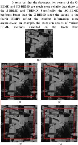
It turns out that the decomposition results of the G-BEMD and SG-G-BEMD are much more reliable than those of the S-BEMD and TBEMD. Specifically, the SG-BEMD performs better than the G-BEMD since the second to the fourth BIMFs reflect the contour information more accurately.As an example, the extension results of various BEMD methods executed on the 167th band
Fig. 3. Extension results (extended length 2V = 32) of different BEMD
methods executed to the 167th band in 92AV3C dataset. (a) Original image.
IJEDR1604124 International Journal of Engineering Development and Research (www.ijedr.org) 838 the original image are symmetrically mapped to the external
parts in the S-BEMD, which are not suitable for handling the asymmetrical image. As displayed in Figs. 6(c) , the extended images in the T-BEMD do not reveal excellent performance though they reflect the developing trend of the original images to a certain extent. For instance, there are large
black areas on the left of the Figs. 6(c) and . Moreover, the boundary extended by the GM(1, Figs. 6(d)significantly verifies the trend of the Fig. 6(a) whereas the images extended by the S-GM(1, 3) Figs. 6(e) ] yield considerable improvements compared with the former methods. Accordingly, the BIMFs and residues of the selected 167th Fig. 6(a)] and 90th bands decomposed by the O-BEMD, S-BEMD, T-S-BEMD, G-BEMD together with the
SG-BEMD are demonstrated in from which it is observed that there exist serious boundary effects in the O-BEMD .
Figure. 3: IEEE 802.15.4 ZigBee stack standard. ZigBee is described by referring to the 7-layers of the OSI model for layered communication systems. The Alliance specifies the bottom three layers Physical, Network, and Data link , as well as Application Programming Interface that allows end developers have the ability to design custom applications that use the services provided by the lower layers. III conclusion
The aim of this paper was to develop a boundary processing strategy to the BEMD and its application to the hyperspectral image classification. To address this issue, the G-BEMD and SG-BEMD, respectively, motivated by the GM (1, 3) and its modified form, i.e., S-GM (1, 3) were proposed in this paper. Regarding the model coefficients and convolution integral are critical factors in the refinement of the MGM, we replaced the existing composite trapezoidal rule with composite.
REFERENCES
1 R. C. Sharpley and V. Vatchev, ―Analysis of the intrinsic mode functions,‖
Constr. Approx., vol. 24, no. 1, pp. 17–47, Apr. 2006. 2 Z. X. Liu and S. L. Peng, ―Directional EMD and its application to texture segmentation,‖ Sci. China Ser. F, vol. 48, no. 3, pp. 354–365, 2005.
3 Z. H. Wu, N. E. Huang, and X. Y. Chen, ―The multi-dimensional ensemble empirical mode decomposition method,‖ Adv. Adap. Data Anal., vol. 1, no. 3, pp. 339–372, 2009.
4 G. L. Xu, X. T. Wang, and X. G. Xu, ―On analysis of bi-dimensional component decomposition via BEMD,‖ Pattern Recogn., vol. 45, no. 4, pp. 1617–1626, Apr. 2012.
5 D. Kim, M. Park, and H. S. Oh, ―Bidimensional statistical empirical
mode decomposition,‖ IEEE Signal Proc. Lett., vol. 19, no. 4, pp. 191–194, Apr. 2012.
6 S. M. A. Bhuiyan, J. F. Khan, and R. R. Adhami, ―A novel approach of edge detection via a fast and adaptive bidimensional empirical mode decomposition method,‖ Adv. Adap. Data Anal., vol. 2, no. 2, pp. 171–192, 2010.
7 Y. Xu, B. Liu, J. Liu, and S. Riemenschneider, ―Two-dimensional empirical mode decomposition by finite elements,‖ Proc. R. Soc. A, vol. 462, no. 2074, pp. 3081–3096, 2006.
8 R. Pabel, R. Koch, G. Jager, and A. Kunoth, ―Fast empirical mode decompositions of multivariate data based on adaptive spline-wavelets and a generalization of the Hilbert– Huang-Transform (HHT) to arbitrary space dimensions,‖ Adv. Adap. Data Anal., vol. 2, no. 3, pp. 337–358, 2010.
9 J. C. Nunes, S. Guyot, and E. Delechelle, ―Texture analysis based on local analysis of the bidimensional empirical mode decomposition,‖ Mach. Vision Appl., vol. 16, no. 3, pp. 177– 188, Feb. 2005.
10 J. C. Nunes, Y. Bouaoune, E. Delechelle, O. Niang, and P. Bunel, ―Image analysis by bidimensional empirical mode decomposition,‖ Image Vision