A Pareto metaheuristic for a bi objective winner determination problem in a combinatorial reverse auction

Munich Personal RePEc Archive

A Pareto-metaheuristic for a bi-objective

winner determination problem in a

combinatorial reverse auction

Buer, Tobias and Kopfer, Herbert

Chair of Logistics, University of Bremen

19 January 2012

Online at

https://mpra.ub.uni-muenchen.de/36062/

Editor

Prof. Dr.-Ing. Herbert Kopfer

Faculty 7: Business Studies & Economics

A Pareto-metaheuristic for a bi-objective winner determination problem

in a combinatorial reverse auction

Tobias Buer and Herbert Kopfer

Working Paper No. 2

All rights reserved by the authors

Prof. Dr.-Ing. H. Kopfer

Chair of Logistics

Faculty 7: Business Studies & Economics

University of Bremen

P.O. Box 33 04 40

28334 Bremen

Germany

Tel.

+49 421 218 66921

Fax

+49 421 218 66922

E-mail

[email protected]

A Pareto-metaheuristic for a bi-objective winner determination problem in a

combinatorial reverse auction

Tobias Buer∗_{, Herbert Kopfer}

Chair of Logistics, University of Bremen, P.O. Box 330440, 28334 Bremen, Germany

Abstract

The bi-objective winner determination problem (2WDP-SC) of a combinatorial procurement auction for transport

contracts comes up to a multi-criteria set covering problem. We are given a setBof bundle bids. A bundle bidb∈B

consists of a bidding carriercb, a bid price pb, and a setτb of transport contracts which is a subset of the setT of

tendered transport contracts. Additionally, the transport qualityqt,cbis given which is expected to be realized when a

transport contracttis executed by a carriercb. The task of the auctioneer is to find a setXof winning bids (X ⊆B),

such that each transport contract is part of at least one winning bid, the total procurement costs are minimized, and

the total transport quality is maximized. This article presents a metaheuristic approach for the 2WDP-SC which

integrates the greedy randomized adaptive search procedure, large neighborhood search, and self-adaptive parameter

setting in order to find a competitive set of non-dominated solutions. The procedure outperforms existing heuristics.

Computational experiments performed on a set of benchmark instances show that, for small instances, the presented

procedure is the sole approach that succeeds to find all Pareto-optimal solutions. For each of the large benchmark

instances, according to common multi-criteria quality indicators of the literature, it attains new best-known solution

sets.

Keywords: Pareto optimization, multi-criteria winner determination, combinatorial auction, GRASP, LNS

1. Introduction and literature review

Combinatorial auctions are applied when bidders are interested in multiple heterogenous items and when the

bidders valuations of these items are non-additive. This is for example the case with the procurement of transport

services which often are highly interdependent. We focus on these kinds of items in the following. In a combinatorial

transport auction, a shipper wants to procure transport services from many freight carriers. Items of a transport auction

are denoted as transport contracts. Such a contract is a framework agreement with a duration of about one to three

years, that defines an origin location and a destination location between which a certain volume of goods has to be

regularly carried (usually on the road) while a specified service level has to be satisfied.

∗_{Corresponding author}

Combinatorial transport auctions allow freight carriers (bidders) to submit bundle bids. Abundle bid is an all-or-nothing bid on any subset of the set of tendered transport contracts. In particular, a freight carrier can bid on

combinations of transport contracts that exhibit strong synergies ([1], [2], [3]). With this, the shipper strives to

reduces his or her total transport costs.

Real-world applications of combinatorial auctions for the procurement of transport service are described by

Led-yard et al. [4], Elmaghraby and Keskinocak [5], for example. Caplice and Sheffi[6, 7] discuss real-world issues of

combinatorial transport auctions and report, among other things, that practical transport auctions studied handle an

average annual procurement volume of 150 million US-dollar. The whole auction process is complex and can last a

few months [6].

After bidding is completed, the shipper (auctioneer) has to decide which of the received bundle bids should be

accepted as winning bids. This problem is known as the winner determination problem which is usually modeled as a

combinatorial optimization problem (for a review see [8]). For combinatorial auctions which are used for selling items,

the set packing problem is used to maximize the total revenue (compare [9, 10], for a review see [11]). Conversely,

the winner determination problem of combinatorial procurement auctions like transport auctions are often modeled

based on the set covering problem or the set partitioning problem and the total procurement costs are minimized.

In practice, shippers usually also want to ensure or improve service quality of the procured transport contracts

(’transport quality’) and therefore do not exploit their full potential for cost savings [3]. Models of winner

deter-mination problems of combinatorial auctions that try to integrate quality aspects in the decision making process are

described in [6], [7], [12], [13]. Primarily, these approaches try to integrate quality aspects as some kind of side

constraint or they use penalty costs to disadvantage low quality carriers or bundle bids, respectively. However, this

requires preference information of the shipper with respect to the desired trade-offbetween transport costs and

trans-port quality. As Caplice and Sheffi [6] state, identifying the desired trade-offis one of the most challenging tasks

in the procurement of transport contracts for a shipper. Therefore, Buer and Pankratz [14] introduced an additional,

second objective function for maximizing the transport quality within a winner determination problem. The resulting

bi-objective model, denoted as 2WDP-SC, seems helpful, if the desired trade-offbetween transport costs and transport

quality is a priori unknown to the shipper.

This paper presents a new heuristic for a bi-objective winner determination problem. The presented heuristic

outperforms previous methods for that optimization problem [14, 15, 16]. The article is organized as follows. Section

2 introduces the studied bi-objective winner determination problem. To solve it, we present a new Pareto metaheuristic

called PNS (Section 3). The performance of PNS is evaluated by means of a benchmark study (Section 4) whose

2. The bi-objective winner determination problem

The bi-objective winner determination problem of a combinatorial transport procurement auction based on a set

covering formulation (2WDP-SC) has been introduced by Buer and Pankratz [14]. We are given a setT of transport contracts offered by a single shipper (decision maker) and a setBof bundle bids which have been submitted by a setCof carriers. A bundle bidb ∈ Bis composed of a carriercb ∈C, a bid price pb ∈ R+, and a subsetτb of the

offered transport contractsT. With the bundle bidb, the carriercb ∈ Cexpresses the intention to execute the set of

transport contractsτb ⊆ T, if he gets paid the price pb by the shipper. Letatb =1 ift ∈ τb andatb =0 otherwise

(∀t∈T,∀b∈B). Ifatb =1, we sayb covers t. Furthermore, we are given parametersqt,cb∈N(∀t∈T,c∈C) which

indicate the achieved transport quality if transport contracttis executed by carriercwho submitted bundle bidb∈B. The shipper prefers higher values ofqt,cb.

The optimization task of the shipper is to determine a set of winning bidsX(X⊆B). The binary decision variable

xbindicates, whether bundle bidb∈Bis accepted as winning bid (xb=1 ⇔b∈X) or not. The 2WDP-SC asks for

the set of winning bidsXthat covers all transport contractsT and at the same time strives to do both, to minimize the total procurement costs and to maximize the total transport quality. The 2WDP-SC is defined by the expressions (1) –

(4).

minf1(X)=

X

b∈B

pb·xb, (1)

minf2(X)=(−1)

X

t∈T

max

b∈B{qt,cb·atb·xb}, (2)

s. t. X

b∈B

atb·xb≥1, ∀t∈T, (3)

xb∈ {0,1}, ∀b∈B. (4)

Objective function f1 (1) minimizes the total procurement costs of the shipper. That is, the sum of the prices of the

winning bids. Objective function f2(2) maximizes the total transport quality of the procured transport contracts. For

ease of notation used later, we minimize the negative total transport quality to obtain a pure minimization problem.

Constraint set (3) guarantees, that each transport contract is covered byat least onewinning bid. Finally, expression (4) ensures, that each bundle bid is an all-or-nothing bid, that is, partial acceptance of a bundle bid is prohibited.

The formulation of the objective function f2 is influenced by the set covering inequality (3). Because of (3), a

transport contracttmay be covered by multiple winning bids although it must be executed only once (this is possible due to the free disposal assumption). Therefore, the maximum function in f2 makes sure, that for each transport

contract t only the highest transport quality valueqt,cb for the given the set of winning bids is summed up once.

Note, that using the set partitioning equality with a strict equal sign instead of (3) would avoid this issue – however,

unwanted by the shipper (using set covering or set partitioning variant in this context is discussed in more detail by

Buer and Pankratz [15, p. 195f]).

The expressions (1), (3), and (4) define the well-known NP-hard set covering problem [17]. If a single objective

decision problem withfk,k=1 is NP-complete, then the corresponding multi objective decision variant with fk,k>1

is also NP-complete [18]. Therefore, the 2WDP-SC is NP-hard.

Finally, we introduce the notation of solution dominance. Let k be the number of objective functions of a minimization problem and let X1,X2 be two feasible solutions. X1 weakly dominates X2, written X1 X2, if

fi(X1)≤ fi(X2),i =1, . . . ,k. X1dominates X2, writtenX1 ≺X2, if fi(X1)≤ fi(X2),i =1, . . . ,kand fi(X1)< fi(X2)

holds at least for onek. An approximation set is a set of feasible solutions which do not≺-dominate each other. The approximation set which contains those feasible solutions which are not weakly dominated by any other feasible

solution is called Pareto-optimal set.

3. A Pareto metaheuristic based on GRASP and adaptive LNS

The developed metaheuristic procedure is denoted as Pareto neighborhood search (PNS). It integrates search

techniques known from the metaheuristics greedy randomized adaptive search procedures (GRASP) and large

neigh-borhood search (LNS). With respect to the multicriteria situation, the search uses dominance-based and

criterion-individual search techniques (cf. Talbi [19, p. 323ff]). Dominance-based search means that values of both objective

functions are used to control the search process, while criterion individual search means that only a single objective

criterion is used and the other is temporarily neglected. An overview of PNS is given in Alg. 1.

Algorithm 1:Pareto neighborhood search (PNS)

Input: problem data: B; parameters:r,dmax,ds Output: approximation setA

A←❞♦♠✐♥❛♥❝❡❇❛s❡❞❈♦♥str✉❝t✐♦♥(B,r,dmax₎

A←❧♦❝❛❧❙❡❛r❝❤(B,ds,A)

3.1. Construction Phase (DRC)

A set of non-dominated solutions is constructed with a method calleddominance-based randomized construction

(DRC, cf. Alg. 2). DRC is a multi start procedure that iteratively constructs feasible solutions to obtain a good

approximation set. The termination of the multi start procedure is controlled by the parameterdmax_{∈N. That is, DRC}

terminates ifdmax_{solutions are constructed successional without finding a new non-dominated solution.}

Algorithm 2:DRC

Input: set of bundle bidsB, no. sectorsr,dmax Output: approximation setA

d←1

repeat ✴✴ r❡st❛rt ❧♦♦♣

k←0

X← ∅

B′←B

whileX infeasibledo

CL← ∅

R1 foreachb∈B\Xdo

if g(b,X)=∞then B←B\ {b}

else

R2 CL←CL⊎ {b}

end

end

b′←s❡❝t♦r❈❛♥❞❙❡❧❡❝t✐♦♥(CL,k,r)

X←X∪ {b′}

k←k+1

end

if(∄X′∈A|X′≺X)then A←A⊎ {X}

d←1

else

d←d+1

end

B←B′ untild=dmax

In thefirst stage, a set of candidate bids, also denoted as candidate listCL ⊂ B\X, is determined. Bids inCL

are potential candidates to be added to the current solutionX. Therefore, we use the vector-valued greedy function

g(b,X)=(P(b,X),Q(b,X)) to rate every bundle bid which was also used by Buer and Pankratz [15]. The elements of

ofg(b,X).

The first rating functionP(b,X) measures the ability of a bundle bidb< Xto makeXa feasible solution and to improve f1(X). Lower values ofP(b,X) are considered as better. P(b,X) calculates the average additional costs for

those contracts inbwhich are not yet covered byX(cf. Chvátal [20]). Letτ(X) denote the set of contracts covered byX, i.e. τ(X)=S

b∈Xτ(b). If all transport contractsτ(b) of a bundle bidbare already covered byX, thenbcannot

contribute to reach feasibility ofXand thereforeP(b,X) is set to+∞.P(b,X) is defined according to (5).

P(b,X)=

             pb

|τ(b)\τ(X)| ifτ(b)\τ(X),∅,

+∞ otherwise.

(5)

The second rating functionQ(b,X) measures the ability of a bundle bidb<Xto improve f2(X). By accepting an

additional bundle bidbas winning bid the transport quality f2 either remains stationary or increases, i.e.,∆f2(X) =

f2(X∪ {b})−f2(X)≥0. In contrast to f1, the value of f2cannot worsen by accepting an additional bid. The increment

in transport quality∆f2(X) is divided by the total number of contracts covered by each individual bid inX∪ {b}, that

isP

b′_∈X∪{b}|τ(b′)|. By this, covering a contract by several bids is penalized. Finally, this value is multiplied by−1, so that smaller values ofQ(b,X) represent better bids (in consistence withP(b,X)). If∆f2(X)=0,bdoes not improve

f2andQ(b,X) assigns a rating of+∞.Q(b,X) is defined according to (6).

Q(b,X)=

            

−_P ∆f2(X)

b′_∈X∪{b}|τ(b′)|

if∆f2(X)>0,

+∞ otherwise.

(6)

By means of the vector-valued rating function g(b,X) the candidate list is constructed during the foreach-loop of

DRC (cf. remark R1 of Alg. 2). As long as the constructed solutionXis infeasible, the following steps are performed: Each bundle bidb ∈ B\Xis rated according to g(b,X). If the rated bundle bidb is not dominated by any of the

bundle bids inCL, thenbis added toCLand those bundle bids inCLwhich are dominated bybare removed. This is symbolized by the operator⊎(cf. remark R2 of Alg. 2). On the other hand, ifg(b,X)=(+∞,+∞) thenbis not able

to contribute to the constructed solutionXand can be disregarded in future ratings of the same solution.

After all bundle bids inB\Xhave been rated and the set of candidate bidsCLis available, a bundle bid has to be selected fromCLand added toXat random. This is done in thesecond stageof the two-stage candidate bid selection procedure.

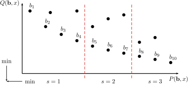
In the second stage, the proceduresectorCandSelect(cf. Alg. 3) selects a particular bundle bidb∈CLthat should be added to the infeasible solutionX. The proceduresectorCandSelectrequires as input the candidate listCL ⊆B, the number of up to now constructed solutionsk∈N, and the external parameterr∈N.

First, the bundle bids of the given candidate listCLare partitioned intorsubsetsCLs⊂CLwhich are denoted as

P(b, x)

Q(b_{, x)}

min min

b1

b2

b3

b4

b5

b6

b7

b8

b9

b10

s= 1 s= 2 s= 3

Figure 1: Organization of candidate list

bundle bidbis randomly chosen with probability 1/|CLs|.

Algorithm 3:sectorCandSelction

Input: candidate listCL, mult start counterk, no. sectorsr Output: a selected bundle bidb,b∈CL

n← |CL|

ifr>nthenr←n

mj← ⌊n/r⌋ ✴✴ ❝❛r❞✐♥❛❧✐t② ♦❢ CLj,1< j<r

m1 ←n−mj·(r−1) ✴✴ ❝❛r❞✐♥❛❧✐t② ♦❢ CL1

sort elements ofCLin increasing order ofP(b,X)

6 s←kmodr+1 ✴✴ ❞❡t❡r♠✐♥❡ s❡❝t♦r

ifs=1then

CLs←CL[1,m1]

else

CLs←CL[m1+mj·(s−2)+1,m1+mj·(s−1)]

end

select a bidb∈CLswith probability 1/|CLs|

returnb

Each sectorCsshould contain an equal number of bundle bids. If an equal division of bids to sectors is not possible

(|CL| modr>0), then the remaining bids are assigned to the first sectorCL1. Therefore,|CL1| ≥ |CL2|=. . .=|CLr|.

In the example of Fig. 1, the candidate listCLis made up of ten non-dominated bundle bidsb1, . . . ,b10. These are

divided intor=3 sectors. SectorCL1contains four bids and sectorsCL2andCL3contain three bids, respectively.

From the sector CLs, a bundle bid is chosen randomly with equal probability. The sectorCLs is determined

from sectorCL2and so forth.

The idea of segmenting the bundle bids into sectors, is to steer the search process into certain dimensions of the

bicriteria objective space. The options to choose a bundle bid in each construction step are reduced and the pressure

to steer into a certain part of the objective space is increased. Without any segmentation (r=1), decisions made in the later stage of constructing a solution might conflict previous decisions. For example, first some bundle bids are chosen

which might result in a good solution with respect to the first objective, later some other bundle bids are chose which

are in favor of the second objective function; sometimes this will lead to good compromise solution but sometimes

the solution quality will be poor in both objective functions.

3.2. Improvement phase

The improvement phase (cf. Alg. 4) is inspired by the metaheuristic large neighborhood search. Basically,

solutions from the approximation setAare destroyed randomly according to a destroy rate and after that rebuilt by means of a greedy single-criterion method. The actual destroy rate and the actual choice of one of the two greedy

rating functionsP(b,X) andQ(b,X) are decided during the improvement phase by setting parameters self-adaptive. The main criterion for the self-adaptive parameter setting, that is the choice of a destroy rate as well as a greedy

rating function, is the number of failed attempts to improveX∈A. This measure for ’success’ of a certain destroy rate and a certain greedy rating function is tracked on a local level for each solution and not on a global level for the entire

approximation set. With this focus on individual solutions inA, the improvement phase is able to better account for structural differences between non-dominated solutions. Structural differences on the decision space level may occur

for solutions that lie in very different areas of the objective space but are nevertheless Pareto optimal. For example, a

solutionXwith a high value for f1(X) and a low value for f2(X) versus a solutionX′with a low value for f1(X′) and a

high value for f2(X′).

The improvement phase (cf. Alg. 4) requires as input an approximation set and a destroy strategy. A destroy

strategydsis a sequencehds1, . . . ,dsniof destroy rates (∀dsi >0). The notationsfail[X].P andfail[X].Q in Alg. 4

denote the number of failed attempts to improve the solutionX with the greedy rating functionP(.,X) and Q(.,X), respectively. Furthermore, the approximation setAis implemented as a first-in, first-out list structure. To remove a solution fromA, the solution on the first position is chosen (cf. remark R1); a new non dominated solutionXis inserted at the back ofA. At the same time, solutions inAwhich are dominated byXare deleted (cf. remark R2). With this first-in, first-out approximation list, the computational effort to improve solutions inAis approximately equally distributed among all regions of the approximation front.

The proceduredestroySol(cf. Alg. 5) destroys a given solution X. This is done by removing bundle bids from

X randomly with a destroy rate (removal probability) of dsi percent. The destroy ratedsi depends on the destroy

Algorithm 4:Improvement phase

Input: approximation setA,ds

repeat

R1 select and remove the first solutionXofA

reinsertXat back ofA

Xd_{←❞❡str♦②❙♦❧✭X,fail[X].P,fail[X].Q,ds✮}

Xr_{←r❡♣❛✐r❙♦❧✭X}d_{,fail[X].P,fail[X].Q✮}

if∄Xa_∈A|Xa_Xr_then

R2 A←A⊎ {Xr} ✴✴ ✐♥s❡rt ❛t ❜❛❝❦ ♦❢ A

fail[Xr].P←0

fail[Xr].Q←0

else iffail[X].P<fail[X].Qthen

fail[X].P←fail[X].P+1

else

fail[X].Q←fail[X].Q+1

end

untiltime limit reached returnA

X′⊆Xwhich is probably infeasible.

Algorithm 5:destroySol

Input: X,fail_P,fail_Q,ds

Output:X′_⊆X

X′_←X

R1 i←min(fail_P,fail_Q) mod|ds|

foreachb∈Xddo

ifrand(1,100)≤dsithenX′←X′\ {b}

end

returnX′

The destroyed solutionX′_{is passed to the procedurerepairSol(cf. Alg. 6). Furthermore, the procedurerepairSol} gets the numbers of failed attemptsfail.P andfail.Q to improveX ⊇X′_{by using rating functionP(.,X) andQ(.,X),} respectively. A new feasible solution is searched for via a a single-criterion greedy heuristic. The heuristic chooses

non-dominated solution (cf. Alg. 6, remark R1). During the while-loop, the solutionX′_{is repaired by consecutively} adding bids toX′ _{in a greedy fashion. If the greedy rating function returns +∞for a bundle bid, this bid cannot} improve the solution and therefore must not be considered in further iterations (cf. Alg. 6, remark R2).

Algorithm 6:repairSol

Input: infeasible solutionX′_{,fail.P,fail.Q}

Output: feasible solutionX⊃X′

R1 iffail.P<fail.Qthen g(., .)←P(., .)

elseg(., .)←Q(., .)

whileX′_infeasibledo

z∗_{← ∞}

b∗_{← ∅ ✴✴ ♠♦st ❣r❡❡❞② ❜✐❞}

foreachb∈B\Xdo ifg(b,X′_)<z∗_then

z∗←g(b,X′)

b∗←b

R2 else ifg(b,X′)=∞thenB←B\ {b}

end

X←X∪ {b∗_}

end

returnX

The improvement phase terminates, after reaching a preset time limit.

3.3. Note on a Mathheuristic Extension

Buer and Pankratz [14] introduced an exact branch-and-bound method based on the epsilon constraint approach

for the 2WDP-SC. This approach, denoted asǫLBB, was successfully used in Buer and Pankratz [15] to hybridize the path-relinking phase of a GRASP method for the 2WDP-SC. Obviously, we therefore also tried to further improve the

solution quality of PNS by integratingǫLBBin three ways: 1) hybridizingǫLBB anddominanceBasedConstruction

(Alg. 2), 2) hybridizingǫLBB andlocalSearch-Phase (Alg. 2), and 3) usingǫLBB in both phases. All in all, given the same computing time, the three hybridized approaches led to inferior results compared to PNS. Therefore, we do

4. Design of computational study

The performance of the proposed heuristic is measured by means of a computational study. This section gives

remarks on the test procedure, presents the used benchmark instances, and introduces measures from the literature for

the quality of an approximation set.

4.1. General remarks and test procedure

The computational evaluation is done by means of artificial benchmark instances. All algorithms were

imple-mented in Java (JDK 6, Update 23). All tests were executed on the same type of personal computer (CPU Intel core

i5-750, four cores a 2.66 GHz). This also includes those heuristics that were published previously (cf. Sect. 5.3), that

is, previous computational experiments were repeated if necessary. Up to four independent computational test runs

were executed in parallel, however, the implementation of the evaluated heuristics uses no parallelization.

We first evaluate some main design choices of the method PNS. At the same time, we work out reasonable values

for the three external parameters of the method PNS. Finally, the new method PNS is compared to three other heuristics

from the literature.

4.2. Benchmark instances

The 37 benchmark instances for the 2WDP-SC introduced by Buer and Pankratz [14] are used. These instances

take into account some specific features of the transportation scenario at hand. In particular, the instance generation

procedure creates bundle bids that satisfy the free disposal assumption. This is important, as this assumption was

required to model the 2WDP-SC with set covering constraints (instead of set partitioning constraints).

For seven instances, all Pareto optimal solutions are known. These instances are denoted as small instances

(instance group S). The small instances feature up to 80 bundle bids. For the remaining thirty instances, the set of

Pareto optimal solutions is unknown. These instances are denoted aslarge instances. These instances are divided into different classes by means of different groups classifying instances according to their number of bundles or their

number of contracts. There are three groups A, B, and C which contain instances with 500, 1000, and 2000 bundle

bids, respectively. The groups a, b, c denote instances with 125, 250, and 500 transport contracts, respectively.

Consequently, the class Cb for example contains those instances with 2000 bundle bids and 250 transport contracts.

This notation is used in Tab. 4, Tab. 5, and Tab. 6.

4.3. Quality indicators for approximation sets

The assessment of the quality of an approximation set is a nontrivial task. An intensive examination of different

approaches is given by Zitzler et al. [21]. The evaluation of algorithms in view of the obtained solution quality is

usually more complex in the multiple objective case than in the single objective case. In the single objective case,

performance statements are naturally made by comparing the objective function values of solutions generated by

each other. Given two approximation setsAandBwith solutions inAthat dominate solutions inBand the other way round (a≺banda′_≺b′_fora,a′_∈Aandb,b′_{∈B) makes performance comparisons difficult.}

One way to measure approximation set quality is the usage of quality indicators which should narrow down

the comparison of two approximation sets to the comparison of two real-valued numbers. Roughly speaking, a

quality indicator is a function that assigns to one or more approximation sets a scalar value. This always goes along

with a loss of information intrinsic to the approximation sets. Hence, it is advisable to use more than one quality

indicator to balance the individual strengths and weaknesses of indicators (which are discussed e.g. by Zitzler et al.

[21]). Therefore, we use three different quality indicators for the computational study, the hypervolume indicator,

the multiplicative epsilon indicator, and the coverage indicator. Those quality indicators seem to be among the most

readily accepted in the literature.

4.3.1. Hypervolume indicator IHV

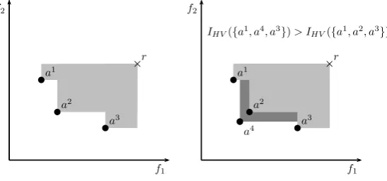
The hypervolume indicatorIHV(A) measures the volume of the objective subspace that is weakly dominated by

the solutions of a given approximation setAand bounded by a reference pointr[22, 23]. The reference pointrhas to be weakly dominated by each solution. Higher indicator values imply a better approximation set. Fig. 2 (left)

shows three non-dominated solutionsa1,a2,a3. The part of the objective space that is dominated by these solutions and bounded by the reference pointris shaded in gray. The volume of the gray area is the value ofIHV({a1,a2,a3}).

In Fig. 2 (right) the new non-dominated solutiona4is added and the hypervolume is increased by the volume of the area shaded in dark gray. Apparently, every new non-dominated solution increases the value ofIHV.

f1 f2 f2 f1 ba 1 ba 2 ba 3 ×r bc a4 ba 1 ba 2 ba 3 ×r

IHV({a1, a4, a3})> IHV({a1, a2, a3})

Figure 2: Principle of hypervolume indicatorIHV.

Following earlier studies on the 2WDP-SC [14, 15], the reference pointris defined asr1= f1(B) andr2=0. The

values of the objective functions f1and f2 differ in several orders of magnitude (using the benchmark instances of

Section 4.2). Therefore they are normalized prior to calculatingIHV according to equation (7).

f_i′(X)= fi(X)−f

min i

ri−fimin

with i∈ {1,2} (7)

andfmin

1 :=0, f

min

4.3.2. Epsilon indicator Iǫ

The multiplicative epsilon indicatorIǫ(A,B) introduced by Zitzler et al. [21, p. 122] compares two approximation

setsAandBand is based on the epsilon dominance relationǫ. It is defined as follows:

f(a)ǫ f(b)⇔ ∀i∈ {1, . . .m}: fi(a)≤ǫ· fi(b). (8)

Iǫ(A,B) is the minimum factor, by which the value of the objective function of each solution in B has to be

multiplied, such that each solution inBis epsilon dominated by at least one solution inA.

Iǫ(A,B)=inf

ǫ∈R{∀b∈B, ∃a∈A: f(a)ǫ f(b)}. (9)

Lower values ofIǫ(A,B) imply a higher quality ofA. By definition, it holds that Iǫ(A,B)≥1. ForIǫ(A,B)=1,

each solution inBis weakly dominated by a solution inA. In general,Iǫ(A,B),Iǫ(B,A) holds.

Iǫ(A,B) is a binary indicator. In case that more than two approximation sets should be compared, a pairwise

comparison of the involved approximation sets is required. To simplify the comparison, in this study, we use the

unary epsilon indicator [24, S. 12]:

Iǫ(A) :=Iǫ(A,AR). (10)

AR _{is denoted as reference approximation set. A}R _{is the set union of the approximation sets A}′_{to be compared} without any dominated solutions.

4.3.3. Coverage indicator IC

Zitzler and Thiele [22, S. 297] introduced the binary coverage indicator. The coverage indicatorIC(A,B) indicates

the fraction of solutions in the approximation setB, that are dominated by at least one solution in the approximation setA.

IC(A,B)=

|{b|∃a∈A: f(a) f(b)}|

|B| . (11)

In general,Iǫ(A,B),Iǫ(B,A) holds. Higher values ofIC(A,B) imply a higher quality ofA. The range of values is

0≤IC(A,B)≤1, whereIC(A,B)=1 indicates, that each solution inBis dominated by at least one solution inA. Like

Iǫ(A,B),IC(A,B) is again a binary indicator and we only use the unary variant by means of a reference approximation

5. Results and discussion

5.1. Contribution of two-stage candidate bid selection

We evaluate, whether the quality of the approximation sets generated by the two-stage candidate bid selection

procedure is improved in comparison to a traditional single-stage bid selection procedure. For this, only the

construc-tion procedure DRC (cf. Alg. 2) is studied. The single-stage selecconstruc-tion procedure is realized by setting the number of

sectorsrto 1. The two-stage procedure is realized by using multiple sectors (r>1).

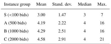
We try to receive an impression of the actual size of the candidate list to identify a reasonable number of sectors

r. Each of the 37 instances was solved 500 times by the heuristic DRC (cf. Alg. 2). Immediately prior to each call of the methodsectorCandSelection(CL,k,r)in DRC, the size of the candidate listCLwas measured. Tab. 1 shows the aggregated results. The average size of the candidate listCLgrows slightly with increasing numbers of bundle bids per instance. Nevertheless, even for the largest instances with 2000 bids, the median of|CL|is only 4 and the maximum size is 21. To avoid an insufficient small number of bids per sector, we use three sectors (r = 3) in the two-stage bid selection approach.

Table 1: Size of the candidate listCLduring construction phase.

Instance group Mean Stand. dev. Median Max.

S (<100 bids) 3.00 1.47 3 7

A (500 bids) 4.19 2.22 4 16

B (1000 bids) 4.29 2.51 4 16

C (2000 bids) 4.58 2.91 4 21

Construction of 500 solutions for each instance.

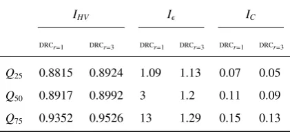
The construction heuristic with a single-stage bid selection is denoted as DRCr=1and the two-stage bid selection

heuristic is denoted as DRCr=3. In contrast to Alg. 2, both heuristics terminate after 1000 constructed solutions (and

dmax_{=∞). For each of the thirty large instances five test runs with different random seeds were performed. A test run}

is the one-time solution of an instance with both heuristics DRCr=1and DRCr=3. The results for the quality indicators

IHV,Iǫ, andICare shown in Tab. 2. Note that approximation setARwas calculated on a per test run basis and not over

all five test runs per instance.

Applying the Wilcoxon signed rank test to the results, the null hypothesis (’the quality indicator median values

of the different algorithms possess the same probability distribution’) can be rejected for each of the three quality

indicators. The p-values forIHV,Iǫ, andICare≤0.0001,≤0.0001, and 0.0028, respectively. The results are statistically

significant even for very tight levels of significance of one percent or lower. Therefore, it is highly likely, that the

observed quality differences of the obtained approximation sets can be attributed to the usage of the two-stage bid

Table 2: One-stage versus two-stage selection of bids from the candidate list with DRCr=1and DRCr=3.

IHV Iǫ IC

DRCr=1 DRCr=3 DRCr=1 DRCr=3 DRCr=1 DRCr=3

Q25 0.8815 0.8924 1.09 1.13 0.07 0.05

Q50 0.8917 0.8992 3 1.2 0.11 0.09

Q75 0.9352 0.9526 13 1.29 0.15 0.13

Regarding the median values of the quality indicatorsIHV andIǫ, the two-stage approach DRCr=3clearly

outper-forms the one-stage heuristic DRCr=1. In contrast, the median values ofICsuggest an opposite interpretation. Looking

at the generated approximation sets, the two-stage heuristic seems to discover better extreme solutions thanDRCr=1,

especially with respect to f1. On the other hand, DRCr=1 seems to generate more and better compromise solutions

with balanced f1and f2values. This might explain the slightly better values ofICin Tab. 2 for the algorithm DRCr=1.

All in all, the two-stage candidate bid selection approach clearly increases the quality of the calculated approximation

sets.

5.2. Contribution of dynamic destroy rates in improvement phase

The goal of this experiment is twofold. On the one hand, we want to check if the proposed dynamic destroy rates

in the solution phase improve approximation set quality. On the other hand, a proper destroy strategy is searched for.

A destroy strategy is a sequencehds1, . . . ,dsniof destroy rates. 17 different destroy strategies are compared, Tab. 3

shows the results. Each of the 17 different destroy strategies is used to compute the thirty large instances twice. These

17 strategies include the five non-dynamic strategiesh3i,h6i,h9i,h12i,h15iwith an a priori fixed destroy rate which is unchangeable. We also experimented with larger destroy rates between 20 and 40 percent, however, these seem

clearly inferior to the smaller destroy rates shown in Tab. 3. Column two to four of Tab. 3 show the median of the

appropriate quality indicator over 60 runs of the destroy strategy. The runtime for each run was fixed to five minutes.

The best median values are bold.

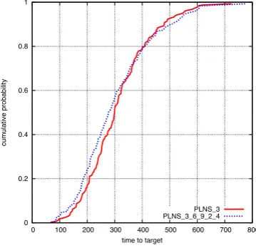
The strategiesh3i, which is static, andh3,6,9,2,4i achieve the best median values for two quality indicators, respectively. We use both strategies to compute each of the large instances five times. Applying the Wilcoxon signed

rank test to the results, the null hypothesis (’the quality indicator median values of the different algorithms possess

the same probability distribution’) can be rejected for two of the three quality indicators on a level of significance of

less than three percent. The p-values forIHV,Iǫ, andIC are≤0.0001, 0.0216, and 0.4231, respectively. The dynamic

strategy clearly outperforms the static strategy by means of the hypervolume indicator while the observed difference

by means of the coverage indicator is not significant. We conclude, that the dynamic strategyh3,6,9,2,4iworks best. Fig. A.3 in the appendix depicts three runtime distributions which indicate that this strategy usually obtains a given

Table 3: Results for 17 different destroy strategies for PLNS.

strategy IHV Iǫ IC

h3,6,9i 0.9095 1.01 0.01

h6,12,18i 0.9093 1.02 0.00

h9,18,27i 0.9089 1.03 0.00

h9,6,3i 0.9097 1.015 0.01

h18,12,6i 0.9096 1.02 0.00

h27,18,9i 0.9093 1.03 0.00

h3i 0.9096 1.01 0.07

h6i 0.9096 1.02 0.02

h9i 0.9096 1.02 0.00

h12i 0.9092 1.025 0.00

h15i 0.9092 1.03 0.00

h5,15,7i 0.9096 1.02 0.00

h7,19,9i 0.9093 1.02 0.00

h15,5,10i 0.9094 1.02 0.00

h19,7,14i 0.9095 1.02 0.00

h3,6,9,2,4i 0.9097 1.01 0.05

h6,12,18,5,10i 0.9096 1.02 0.00

5.3. Comparison with other heuristics

To benchmark the new method PNS by means of approximation set quality the three heuristics SPEA2A,

P-GRASPP+HPR, and PGRASPQ+HPR are used. The method SPEA2A is based on theStrength Pareto Evolutionary

Algorithm 2 introduced by Zitzler et al. [25]. This generic multi objective genetic algorithm wasadapted by ge-netic operators specific to the 2WDP-SC in [14]. In that paper the method was called A8. PGRASPP+HPR, and

PGRASPQ+HPR were proposed in [15]. Both methods are multi objective GRASP whose path-relinking phase was

hybridized with the exact branch-and-bound methodǫLBBby [14]. Another hybridized heuristic for the 2WDP-SC was discussed in [16] (see also 3.3) which is, however, not included in our comparison, as it does not clearly

outperform the mentioned heuristics on the majority of instances.

For the benchmark, the parameters of PNS are set as follows. The number of sectionsrare set to 3, the vector destroy probabilities is set to (3,6,9,2,4), and the termination criterion of the construction phase is set todmax _=92.

While the configuration of the first two values were justified in Sections 5.1 and 5.2, the value of the termination

criteriondmax_{was determined as follows: for each large instance, 1000 solutions were generated with DRC (cf. Alg.}

2). The experimental distribution of the number of unsuccessful improvement tries was recorded (median 6, mean 20,

standard deviation 42) anddmax_{was set to the value of the ninety-five percent quantile, which is 92.}

The runtime of each heuristic was five minutes (300s). All heuristics solved all instances on the same type of

computer. Please note, wedo not citethe computational results of the experiments in [14, 15] but solve all instances again on the same (and faster) computer.

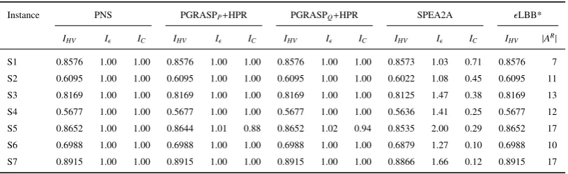
The results for the small instances with known Pareto optimal solution sets are shown in Tab. 4. The two rightmost

columns show the Pareto optimal hypervolume values and the cardinality of the reference approximation setAR_(here,

it is identical to the Pareto optimum solution set). These optimal results haven been obtained by the bicriteria

branch-and-bound methodǫLBBintroduced in [14].

Algorithm PNS is able to solve all seven small instances to Pareto optimality, that is the whole Pareto optimal

solution set is found. In contrast, the procedures PGRASPP+HPR and PGRASPQ+HPR are able to solve six out of

seven instances to Pareto optimality. In [15], only four instances could be solved to Pareto optimality. The method

SPEA2A is able to find some Pareto optimal solutions for six instances (S1 – S5, S7), but never the complete set.

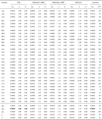
The results for the large instances without known Pareto optimum solution are shown in Tab. 5. This time, the

reference approximation setAR(cf. two rightmost columns) is generated by merging the approximation sets of PNS, PGRASPP+HPR, PGRASPQ+HPR, and SPEA2A and removing the dominated solutions. The last five rows of Tab.

5 show the 25 percent quantile, the median, the 75 percent quantile, the mean, and the standard deviation for each

heuristic and each quality indicator.

The heuristic PNS finds new best approximation sets in terms of IHV andIǫ for all thirty instances. Therefore,

PNS clearly outperforms the existing approaches in terms of approximation set quality. Furthermore, from the values

ofICfollows that the approximation sets computed by PNS are even equal to the reference approximation setAR in

Table 4: Comparison of solution approaches by means of small instances (instance group S).

Instance PNS PGRASPP+HPR PGRASPQ+HPR SPEA2A ǫLBB*

IHV Iǫ IC IHV Iǫ IC IHV Iǫ IC IHV Iǫ IC IHV |AR|

S1 0.8576 1.00 1.00 0.8576 1.00 1.00 0.8576 1.00 1.00 0.8573 1.03 0.71 0.8576 7

S2 0.6095 1.00 1.00 0.6095 1.00 1.00 0.6095 1.00 1.00 0.6022 1.08 0.45 0.6095 11

S3 0.8169 1.00 1.00 0.8169 1.00 1.00 0.8169 1.00 1.00 0.8125 1.47 0.38 0.8169 13

S4 0.5677 1.00 1.00 0.5677 1.00 1.00 0.5677 1.00 1.00 0.5636 1.41 0.25 0.5677 12

S5 0.8652 1.00 1.00 0.8644 1.01 0.88 0.8652 1.02 0.94 0.8535 2.00 0.29 0.8652 17

S6 0.6988 1.00 1.00 0.6988 1.00 1.00 0.6988 1.00 1.00 0.6879 1.27 0.10 0.6988 10

S7 0.8915 1.00 1.00 0.8915 1.00 1.00 0.8915 1.00 1.00 0.8866 1.66 0.12 0.8915 17

*The methodǫLBB calculates always Pareto-optimal solutions.

by PNS. Consequently, the solution approach PNS obtains for all three quality indicators the best median indicator

values at the same time.

5.4. Runtime behavior

To compare the runtime of the three heuristics from the literature with the new method PNS, a target hypvervolume

value is defined for each instance. The runtime needed to achieve the target value is measured.

The target value is defined as the lowestIHVvalue per instance shown in Tab. 4 and Tab. 5. Therefore, we are sure

that each heuristic has been able to reach the target value at least once. The best known hypervolume value seems not

to be a qualified target value because this target value will probably not be reached by most heuristics, which limits

the value of the experiment. Following, each instance is solved by each heuristic 75 times and the time to target is

measured. The total runtime per heuristic was limited to three minutes (180s). Note, if an algorithm could not reach

the target value within 180s, then a runtime of 180s is reported anyway. Therefore, an algorithm might appear faster

than it actually is. However, this behavior occurred only with the heuristic SPEA2A and never with the heuristic PNS.

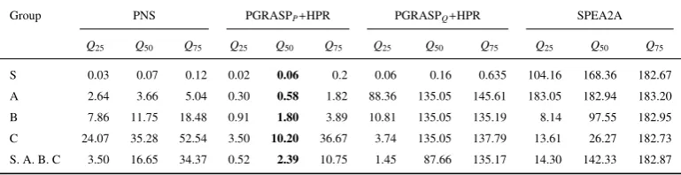
The aggregated results are reported in Tab. 6. According to the reported median values for the 37 instances, the

new heuristic PNS ranks second. The fastest method is PGRASPP+HPR, third place goes to PGRASPQ+HPR, and

fourth place goes to SPEA2A. The median runtime of the method PGRASPQ+HPR for the larger instances is around

135s, which can be explained by a switch from the neighborhood search phase towards the path relinking phase, which

is time dependent. Furthermore, although SPEA2A can repeatedly not achieve the target value in the predefined 180s

(cf.Q75in Tab. 6), for some of the larger instances SPEA2A seems competitive (cf.Q25andQ50).

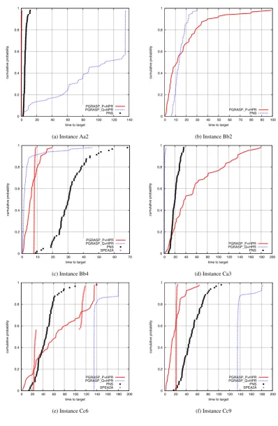
To give more insights into the runtime behavior of the heuristics, Fig. A.4(a)-(f) show the experimental runtime

distribution for selected instances. The method SPEA2A is missing on some figures, as this procedure is sometimes

Table 5: Comparison of solution approaches by means of large instances (instance groups A, B, and C).

Instance PNS PGRASPP+HPR PGRASPQ+HPR SPEA2A reference

IHV Iǫ IC IHV Iǫ IC IHV Iǫ IC IHV Iǫ IC IHV |AR|

Aa1 0.9027 1.00 1.00 0.8996 1.14 0.00 0.8929 1.11 0.00 0.8895 1.33 0.00 0.9027 68

Aa2 0.9132 1.00 1.00 0.9118 1.06 0.00 0.9056 1.09 0.00 0.9016 1.42 0.00 0.9132 43

Aa3 0.9063 1.00 1.00 0.9026 1.04 0.00 0.8996 1.08 0.00 0.8979 1.29 0.00 0.9063 60

Ba1 0.9559 1.00 1.00 0.9521 1.21 0.00 0.9510 1.13 0.00 0.9475 1.43 0.00 0.9559 100

Ba2 0.9596 1.00 1.00 0.9578 1.11 0.00 0.9545 1.14 0.00 0.9502 1.85 0.00 0.9596 80

Ba3 0.9619 1.00 0.99 0.9595 1.22 0.00 0.9557 1.19 0.01 0.9521 1.36 0.00 0.9619 70

Bb1 0.9084 1.00 1.00 0.9050 1.17 0.00 0.9013 1.08 0.00 0.8971 1.34 0.00 0.9084 58

Bb2 0.9070 1.00 1.00 0.9036 1.13 0.00 0.9009 1.07 0.00 0.8990 1.29 0.00 0.9070 65

Bb3 0.9050 1.00 1.00 0.9033 1.14 0.00 0.8984 1.07 0.00 0.8960 1.33 0.00 0.9050 51

Bb4 0.9143 1.00 1.00 0.9071 1.36 0.00 0.9024 2.00 0.00 0.8840 20.00 0.00 0.9143 149

Bb5 0.9071 1.00 1.00 0.9006 1.12 0.00 0.8988 1.10 0.00 0.8913 2.00 0.00 0.9071 108

Bb6 0.9102 1.00 1.00 0.9041 1.24 0.00 0.8993 1.13 0.00 0.8941 1.35 0.00 0.9102 114

Ca1 0.9809 1.00 1.00 0.9798 1.21 0.00 0.9783 1.18 0.00 0.9579 11.00 0.00 0.9809 100

Ca2 0.9825 1.00 1.00 0.9809 1.35 0.00 0.9794 1.22 0.00 0.9793 1.53 0.00 0.9825 85

Ca3 0.9812 1.00 1.00 0.9781 2.00 0.00 0.9786 1.17 0.00 0.9691 5.00 0.00 0.9812 73

Cb1 0.9585 1.00 1.00 0.9560 1.15 0.00 0.9529 1.15 0.00 0.9527 1.27 0.00 0.9585 78

Cb2 0.9589 1.00 1.00 0.9567 1.21 0.00 0.9539 1.13 0.00 0.9527 1.35 0.00 0.9589 50

Cb3 0.9569 1.00 1.00 0.9544 1.09 0.00 0.9530 1.09 0.00 0.9512 1.32 0.00 0.9569 30

Cb4 0.9594 1.00 1.00 0.9546 2.00 0.00 0.9533 1.17 0.00 0.9410 13.00 0.00 0.9594 143

Cb5 0.9621 1.00 1.00 0.9581 1.42 0.00 0.9556 1.19 0.00 0.9495 7.00 0.00 0.9621 119

Cb6 0.9586 1.00 1.00 0.9537 1.33 0.00 0.9524 1.17 0.00 0.9507 1.54 0.00 0.9586 100

Cc1 0.8991 1.00 1.00 0.8914 2.00 0.00 0.8883 1.11 0.00 0.8773 27.00 0.00 0.8991 147

Cc2 0.9083 1.00 1.00 0.8980 3.00 0.00 0.8974 1.15 0.00 0.8894 16.00 0.00 0.9083 164

Cc3 0.9043 1.00 1.00 0.8972 1.30 0.00 0.8944 1.11 0.00 0.8923 1.29 0.00 0.9043 128

Cc4 0.9087 1.00 1.00 0.9059 1.03 0.00 0.9046 1.05 0.00 0.9013 1.20 0.00 0.9087 14

Cc5 0.9014 1.00 1.00 0.8996 1.02 0.00 0.8980 1.04 0.00 0.8972 1.05 0.00 0.9014 8

Cc6 0.8980 1.00 1.00 0.8962 1.02 0.00 0.8949 1.03 0.00 0.8931 1.21 0.00 0.8980 12

Cc7 0.9001 1.00 0.97 0.8940 1.09 0.00 0.8923 1.08 0.03 0.8916 1.23 0.00 0.9001 86

Cc8 0.9042 1.00 1.00 0.8981 1.19 0.00 0.8955 1.09 0.00 0.8957 1.23 0.00 0.9042 65

Cc9 0.9018 1.00 1.00 0.8932 1.11 0.00 0.8922 1.10 0.00 0.8905 1.22 0.00 0.9018 89

Q25 0.9045 1.00 1.00 0.8996 1.11 0.00 0.8976 1.08 0.00 0.8925 1.29 0.00 0.9045 59

Q50 0.9095 1.00 1.00 0.9055 1.18 0.00 0.9019 1.11 0.00 0.8985 1.35 0.00 0.9095 79

Q75 0.9588 1.00 1.00 0.9557 1.32 0.00 0.9532 1.17 0.00 0.9506 1.96 0.00 0.9588 106

µ 0.9292 1.00 1.00 0.9251 1.32 0.00 0.9225 1.15 0.00 0.9178 4.35 0.00 0.9292 82

σ 0.0303 0.00 0.01 0.0315 0.42 0.00 0.0320 0.17 0.01 0.0315 6.50 0.00 0.0303 41

Q50denotes the median. The best median-values are bold.Q25andQ75denote the lower and upper quartile, respectively.

Table 6: Comparison of the runtime (s) of the four heuristics for instance groups S, A, B, and C.

Group PNS PGRASPP+HPR PGRASPQ+HPR SPEA2A

Q25 Q50 Q75 Q25 Q50 Q75 Q25 Q50 Q75 Q25 Q50 Q75 S 0.03 0.07 0.12 0.02 0.06 0.2 0.06 0.16 0.635 104.16 168.36 182.67

A 2.64 3.66 5.04 0.30 0.58 1.82 88.36 135.05 145.61 183.05 182.94 183.20

B 7.86 11.75 18.48 0.91 1.80 3.89 10.81 135.05 135.19 8.14 97.55 182.95

C 24.07 35.28 52.54 3.50 10.20 36.67 3.74 135.05 137.79 13.61 26.27 182.73

S. A. B. C 3.50 16.65 34.37 0.52 2.39 10.75 1.45 87.66 135.17 14.30 142.33 182.87

6. Conclusion

Considering quality aspects during winner determination in a combinatorial reverse auction for transport contracts

is of practical importance. In this paper, we studied a bi-objective winner determination problem that is based on the

set covering problem and minimizes the total transport costs and the total transport quality simultaneously. To solve

this problem, the heuristic PNS was developed. PNS is inspired by the metaheuristics GRASP and LNS. To construct

an initial set of non dominated solutions, PNS applies a dominance-based randomized greedy heuristic which uses

a two-stage candidate bid selection procedure. The initial solutions are improved by means of a search in large

neighborhoods which switches the applied parameters (removal probability of bids and greedy rating function) in a

self-adaptive manner. Self-adaptive configurations depend on individual solutions and not on the entire approximation

set. PNS was tested by means of 37 benchmark instances. In terms of approximation set quality, PNS outperforms

all known heuristics on each of the 37 benchmark instances. Furthermore, PNS is the second fastest method tested.

Subject of our future research will be the development of solution approaches for bi-objective winner determination

problems which take into account additional business constraints proposed e.g. by Caplice and Sheffi[6].

Appendix A. Time-to-Target plots

Hoos and Stützle [26] as well as Ribeiro et al. [27] discuss the evaluation of algorithms by runtime distributions.

Time to targetplots were introduced by Feo et al. [28]. To draw the plots presented in this appendix the programm of Aiex et al. [29] was used.

References

[1] Kopfer H, Pankratz G. Das Groupage-Problem kooperierender Verkehrsträger. In: Kall P, Lüthi HJ, editors. Operations Research Proceedings

1998. Berlin: Springer; 1999, p. 453–62.

[2] Pankratz G. Analyse kombinatorischer Auktionen für ein Multi-Agentensystem zur Lösung des Groupage-Problems kooperierender

Spedi-tionen. In: Inderfurth K, Schwödiauer G, Domschke W, Juhnke F, Kleinschmidt P, Wäscher G, editors. Operations Research Proceedings

1999. Berlin: Springer; 2000, p. 443–8.

0 0.2 0.4 0.6 0.8 1

0 100 200 300 400 500 600 700 800 900 1000

cumulative probability

time to target

PLNS_3 PLNS_3_6_9_2_4

(a) Instance Aa2, target valueIHV=0.9131

0 0.2 0.4 0.6 0.8 1

0 100 200 300 400 500 600 700 800 900 1000

cumulative probability

time to target

PLNS_3 PLNS_3_6_9_2_4

(b) Instance Bb6, target valueIHV=0.9097

0 0.2 0.4 0.6 0.8 1

0 100 200 300 400 500 600 700 800

cumulative probability

time to target

PLNS_3 PLNS_3_6_9_2_4

(c) Instance Cc5, target valueIHV=0.9046

0 0.2 0.4 0.6 0.8 1

0 20 40 60 80 100 120 140

cumulative probability

time to target

PGRASP_P+HPR PGRASP_Q+HPR PNS

(a) Instance Aa2

0 0.2 0.4 0.6 0.8 1

0 10 20 30 40 50 60 70 80 90 100

cumulative probability

time to target

PGRASP_P+HPR PNS

(b) Instance Bb2

0 0.2 0.4 0.6 0.8 1

0 10 20 30 40 50 60 70

cumulative probability

time to target

PGRASP_P+HPR PGRASP_Q+HPR PNS SPEA2A

(c) Instance Bb4

0 0.2 0.4 0.6 0.8 1

0 20 40 60 80 100 120 140 160 180 200

cumulative probability

time to target

PGRASP_P+HPR PGRASP_Q+HPR PNS

(d) Instance Ca3

0 0.2 0.4 0.6 0.8 1

0 20 40 60 80 100 120 140 160 180 200

cumulative probability

time to target

PGRASP_P+HPR PGRASP_Q+HPR PNS SPEA2A

(e) Instance Cc6

0 0.2 0.4 0.6 0.8 1

0 20 40 60 80 100 120 140 160 180 200

cumulative probability

time to target

PGRASP_P+HPR PGRASP_Q+HPR PNS SPEA2A

(f) Instance Cc9

[4] Ledyard JO, Olson M, Porter D, Swanson JA, Torma DP. The first use of a combined-value auction for transportation services. Interfaces

2002;32(5):4–12.

[5] Elmaghraby W, Keskinocak P. Combinatorial auctions in procurement. In: Harrison T, Lee H, Neale J, editors. The Practice of Supply Chain

Management: Where Theory and Application Converge. New York: Springer-Verlag; 2004, p. 245–58.

[6] Caplice C, SheffiY. Combinatorial auctions for truckload transportation. In: Cramton P, Shoaham Y, Steinberg R, editors. Combinatorial

Auctions. Cambridge, MA: MIT Press; 2006, p. 539–71.

[7] Caplice C, SheffiY. Optimization-based procurement for transportation services. Journal of Business Logistics 2003;24(2):109–28.

[8] Abrache J, Crainic T, Gendreau M, Rekik M. Combinatorial auctions. Annals of Operations Research 2007;153(34):131–64.

[9] Goossens D, Spieksma F. Exact algorithms for the matrix bid auction. Computers & Operations Research 2009;36(4):1090 –109.

[10] Yang S, Segre AM, Codenotti B. An optimal multiprocessor combinatorial auction solver. Computers & Operations Research 2009;36(1):149

–66.

[11] de Vries S, Vohra RV. Combinatorial auctions: A survey. INFORMS Journal on Computing 2003;15(3):284–309.

[12] Catalán J, Epstein R, Guajardo M, Yung D, Martínez C. Solving multiple scenarios in a combinatorial auction. Computers & Operations

Research 2009;36(10):2752 –8.

[13] Chen RLY, AhmadBeygi S, Cohn A, Beil DR, Sinha A. Solving truckload procurement auctions over an exponential number of bundles.

Transportation Science 2009;43(4):493–510.

[14] Buer T, Pankratz G. Solving a bi-objective winner determination problem in a transportation procurement auction. Logistics Research

2010;2(2):65–78.

[15] Buer T, Pankratz G. Grasp with hybrid path relinking for bi-objective winner determination in combinatorial transportation auctions. Business

Research 2010;3(2):192–213.

[16] Buer T, Kopfer H. Shipper decision support for the acceptance of bids during the procurement of transport services. In: Böse J, Hu H, Jahn

C, Shi X, Stahlbock R, Voß S, editors. Proceedings of the 2nd International Conference on Computational Logistics (ICCL’11); vol. 6971 of

LNCS. Springer; 2011, p. 18–28.

[17] Karp RM. Reducibility among combinatorial problems. In: Miller RE, Thatcher JW, editors. Complexit of Computer Computations. New

York: Plenum Press; 1972, p. 85–103.

[18] Serafini P. Some considerations about computational complexity for multi objective combinatorial problems. In: Jahn J, Krabs W, editors.

Recent advances and historical development of vector optimization; vol. 294 ofLecture Notes in Economics and Mathematical Systems.

Berlin, Germany.: Springer-Verlag; 1986, p. 222–32.

[19] Talbi EG. Metaheuristics – From Desing to Implementation. Hoboken, New Jersey, USA: Wiley-Verlag; 2009.

[20] Chvátal V. A greedy heuristic for the set-covering problem. Mathematics of Operations Research 1979;4(3):233–5.

[21] Zitzler E, Thiele L, Laumanns M, Fonseca CM, da Fonseca VG. Performance assessment of multiobjective optimizers: An analysis and

review. IEEE Transactons on Evolutionary Computation 2003;7:117–32.

[22] Zitzler E, Thiele L. Multiobjective optimization using evolutionary algorithms - a comparative case study. In: Eiben A, Bäck T, Schoenauer

M, Schwefel HP, editors. Parallel Problem Solving from Nature – PPSN V; vol. 1498 ofLNCS. Springer Berlin/Heidelberg; 1998, p.

292–301.

[23] Zitzler E, Thiele L. Multiobjective evolutionary algorithms: A comparative case study and the strength Pareto approach. IEEE Transactions

on Evolutionary Computation 1999;3(4):257–71.

[24] Knowles JD, Thiele L, Zitzler E. A tutorial on the performance assessment of stochastic multiobjective optimizers. TIK-Report 214;

Computer Engineering and Networks Laboratory, ETH Zurich; 2006.

[25] Zitzler E, Laumanns M, Thiele L. SPEA2: Improving the strength Pareto evolutionary algorithm. TIK-Report 103; Federal Institute of

Technology (ETH) Zurich, Zurich (2001); 2001.

[26] Hoos HH, Stützle T. Towards a characterisation of the behaviour of stochastic local search algorithms for SAT. Artificial Intelligence

[27] Ribeiro C, Rosseti I, Vallejos R. On the use of run time distributions to evaluate and compare stochastic local search algorithms. In: Stützle T,

Birattari M, Hoos H, editors. Engineering Stochastic Local Search Algorithms. Designing, Implementing and Analyzing Effective Heuristics;

vol. 5752 ofLNCS. Springer-Verlag; 2009, p. 16–30.

[28] Feo TA, Resende MG, Smith SH. A greedy randomized adaptive search procedure for maximum independent set. Operations Research

1994;42(5):860–78.