A first attempt on global evolutionary undersampling for imbalanced big data

A First Attempt on Global Evolutionary Undersampling for

Imbalanced Big Data

I. Triguero, M. Galar, H. Bustince, F. Herrera

Abstract— The design of efficient big data learning models has become a common need in a great number of applications. The massive amounts of available data may hinder the use of traditional data mining techniques, especially when evolution-ary algorithms are involved as a key step. Existing solutions typically follow a divide-and-conquer approach in which the data is split into several chunks that are addressed individually. Next, the partial knowledge acquired from every slice of data is aggregated in multiple ways to solve the entire problem. However, these approaches are missing a global view of the data as a whole, which may result in less accurate models.

In this work we carry out a first attempt on the design of a global evolutionary undersampling model for imbalanced classification problems. These are characterised by having a highly skewed distribution of classes in which evolutionary models are being used to balance it by selecting only the most relevant data. Using Apache Spark as big data technology, we have introduced a number of variations to the well-known CHC algorithm to work very large chromosomes and reduce the costs associated to fitness evaluation. We discuss some preliminary results, showing the great potential of this new kind of evolutionary big data model.

I. INTRODUCTION

Learning from big datasets is a great challenge for most machine learning techniques. Although they are supposed to work better when there is an abundance of data to leverage their outcome, in practice, they cannot be really applied due to memory and time limitations [1]. New parallelisation technologies, however, provide us powerful tools to handle large amounts in the form of distributed datasets [2]. Thus, the problem now consists of figuring out the most suitable way of using such technology to come up with effective learning algorithms.

Hadoop [3] and the MapReduce paradigm [4] served as the first alternatives to deal with data-intensive kind of applica-tions. The key point lied in the use of a distributed file system that allowed us to parallelise multiple tasks across a cluster of compting nodes in a transparent and fault-tolerant manner [5]. Soon enough, the machine learning community found multiple limitations [6] to deploy efficiently algorithms that share data across multiple stages (e.g. iterative algorithms).

This work was supported by the Research Projects TIN2014-57251-P and TIN2016-77356-P

I. Triguero is with the School of Computer Science, University of Nottingham, United Kingdom. E-mail: [email protected]

F. Herrera is with the Department of Computer Science and Artificial Intelligence of the University of Granada, CITIC-UGR, Granada, Spain, 18071. E-mail: [email protected]

M. Galar and H. Bustince are with the Department of Automatics and Computation, Universidad P ´ublica de Navarra, Campus Arrosad´ıa s/n, 31006 Pamplona, Spain. E-mails:{mikel.galar, bustince}@unavarra.es

New platforms such as Spark [2] or Flink [7] build upon the MapReduce paradigm, providing us a new kind of high throughput in-memory distributed datasets that easily allow us to repeatedly carry out operations on the data.

Multiple MapReduce-like strategies have been developed to adapt traditional machine learning and data mining tech-niques to the new big data scenario. Most of these methods are approximations of the original algorithms, and just a few of them are exact replicas of the sequential version. Approximate models typically divide the data into smaller subsets in which the original algorithm is applied. Then, the different outcomes from each part are somehow combined [8]. Global or exact approaches aim to replicate the behaviour of the sequential version by letting it see the data as a whole (and not as a combination of smaller parts). As an example, we can find the Decision Trees implemented in Apache Spark [2] or the big data version of the k-nearest neighbours proposed in [9]. The great advantage of this last approach is that they may become more robust and precise, but they tend to be slower.

Even when there are lots amounts of data, we may also run into the situation where there is scarcity of a particular class of samples. Focusing on two-class problems, this issue is known as the class imbalance problem [10], in which positive data samples (usually the class of interest) are highly outnumbered by negative ones [11]. It brings along a series of difficulties such as overlapping, small sample size, or small disjuncts [12]. Several approaches have been designed to tackle this problem, which can be divided into three main groups: data sampling, algorithmic modifications and cost-sensitive solutions. These models have been also successfully combined with ensemble learning algorithms [13].

Evolutionary undersampling (EUS) [14] belongs to the data sampling family of methods, where the main objective is to balance the distribution of classes of the original dataset by removing examples of the negative class. This removal is carefully guided by a genetic-based algorithm that aims to increase the performance on the two classes of the problem. However, dealing with a large number of negative examples would lead to a high chromosome size, resulting in a huge search space that limits the straightforward application of EUS on big data. In previous works [15], [16], we devised approximate approaches, based on Hadoop and Spark tech-nologies, that split the original problem into small pieces in which EUS could be applied concurrently. Despise their performance, these models lack of a global view of the entire dataset.

global EUS is feasible with the current technology, in terms of runtime and in comparison to approximate models. As new technologies, such as Spark, allow us to take multiple iterations over the same data without a heavy penalty, we can now devise a parallel EUS that basically distributes time consuming and high memory demanding operations across a number of worker processes, while the main procedure would be running in the driver process. As evolutionary algorithm, we focus on the widely-used CHC evolutionary algorithm [17], which is modified to create a more compact repre-sentation of the chromosomes, and make use of distributed datasets when evaluating the current population.

The paper is structured as follows. Section II provides background information about evolutionary undersampling for imbalanced big data classification. Section III discusses the decisions made to take the CHC model to the big data context with Apache Spark. Section IV analyses the empiri-cal results. Finally, Section V summarises the conclusions.

II. BACKGROUND

This section briefly describes the big data technologies used in this paper (Section II-A) as well as the current state-of-the-art on imbalanced big data classification (Section II-B).

A. Big Data Technologies

The MapReduce programming paradigm [4] is a scalable data processing tool designed by Google in 2003. It was designed to be part of the most powerful search-engine on the Internet, but it rapidly became one of the most effective techniques for general-purpose data intensive applications.

Apache Hadoop [18] is the most popular open-source implementation of MapReduce. It is widely used because of its performance, open source nature, installation facilities and its distributed file system (Hadoop Distributed File System, HDFS). Despite its popularity, Hadoop and MapReduce cannot deal with online or iterative computing, producing significant computational costs to reuse the data.

Apache Spark is a novel solution large-scale data process-ing to solve the drawbacks of Hadoop. Spark is part of the Hadoop Ecosystem and it uses the HDFS. This framework proposes a set of in-memory primitives, beyond the stan-dard MapReduce, aiming at processing data more rapidly on distributed environments. Spark is based on Resilient Distributed Datasets (RDDs), a special type of data structure used to parallelize the computations in a transparent way. These parallel structures let us persist and reuse results efficiently, since they are cached in memory. Moreover, they also let us manage the partitioning to optimize data placement, and manipulate data using transparent primitives. Very recently, Spark is moving towards even more eficient APIs such as DataFrame and Datasets.

B. Imbalanced classification in the Big Data context

In a binary classification scenario a dataset is said to be imbalanced whenever the number of instances of one class outnumbers that of the other. In this situation, performance

measures like the accuracy rate (percentage of correctly classified examples) are no longer valid to measure the quality of the models obtained, since the performance over both classes is not equally weighted. Two commonly used alternatives are the Area Under the ROC Curve (AUC) and the g-mean.

The AUC (Area Under the ROC-Curve) [19] provides a scalar value measuring how well a classifier trades off its true positive (TPrate) and false positive rates (FPrate). A popular approximation [10] of this measure is given by

AU C= 1 + TPrate₂−FPrate. (1) Similarly, the g-mean is the acronym for the geometric mean. In this case, the balance between the true positive rates and true negative rates (TNrate) of the classifier is measured, that is, how well the classifier is able to recognize both classes at the same time:

g-mean =TPrate·TNrate (2)

These two measures have been extensively and interchange-ably used in various experimental studies of imbalanced classification [10], [14].

Any classification problem can be affected by the pres-ence of class imbalance, and big data problems are not an exception. Even though the quantity of data is much bigger, the imbalance ratio (the number of majority class examples divided by the number of negative class examples) can still be to high so as to extract meaningful models. One main drawback of distributing large imbalanced datasets across different nodes is that the sample size of the minority class in each node will become lower. As a consequence, when a local model is learned using only a subset of the training set, the presence of too little minority class examples can end hindering the classifier learning phase as it is one of the main sources of problems in imbalanced domains [10].

EUS is an interesting alternative to deal with big data imbalanced problems as it reduces the dataset size, on the contrary to oversampling methods that generate even more data [20]. Hence, the corresponding model can be built faster. Another way of reducing the dataset size is by means of ran-dom undersampling (RUS). However, its main disadvantage is that it could discard important data from the majority class due to the random nature behind its functioning procedure, whereas EUS guides the balancing of the dataset to preserve or even improve the final performance.

Several data level algorithms were tested in [20] to deal with imbalanced big data classification problems (random over/undersampling and SMOTE). Afterwards, a Random Forest classifier [21] was trained. A different approach was taken in [22] where a fuzzy rule-based classification system was developed to address the class imbalance problem in the big data context. In order to do so, the authors proposed a cost-sensitive approach developed over the MapReduce adaptation of the fuzzy classifier.

two-Fig. 1: EUS local for extremely imbalanced datasets [16]

level parallelization model where MapReduce was used to divide the problem into smaller subproblems over which EUS was applied and a windowing scheme was used to reduce the evaluation of each chromosome in each node. However, the small-sample size problem was not addressed in this first approach due to the limitations of Hadoop framework. Nevertheless, this was the main focus of their subsequent work [16], where the authors took advantage of the primitives provided by Spark to properly deal with the small-sample size problem. Spark allows one to broadcast a set of data to all the nodes. This useful property was used to broadcast all the minority class examples to all the nodes so that EUS and the corresponding decision tree could make use of the whole minority class information. In this work, our aim is to go one step further using all the potential offered by Spark to develop a first attempt of a global EUS model. This way, we will be able not only to get rid of the small-sample size problem, but also to obtain a reduced set which is selected considering the dataset as a whole, which has not been developed before.

III. AGLOBAL EVOLUTIONARY UNDERSAMPLING FOR IMBALANCED BIG DATA WITHAPACHESPARK

In this section we describe the proposed global EUS for imbalanced big datasets based on Apache Spark. We discuss the necessary changes made to the original EUS proposal to extend it to the big data context.

EUS [14] was devised as a new kind of evolutionary instance selection algorithm [23] that accounts for the class imbalance problem. The focus of EUS is to balance the dataset in such a way that the performance is maximised in both classes of the problem.

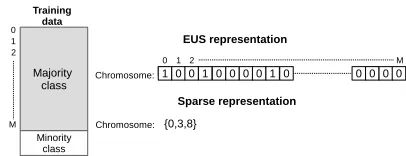
Following the general procedure of an evolutionary al-gorithm, it starts off with a population of N P candidate solutions. In the original EUS, a binary chromosome is used to encode every possible solution. In this chromosome, each bit represents the presence (1) or absence (0) of an instance in the training set. To reduce the search space, only majority class instances are considered for removal, including always all the minority class instances in the final dataset.

Having a set ofM majority class instances, the first issue we encounter when dealing with big datasets (i.e.M is very big) is that this chromosome will be extremely big as it is representing every single majority class instance. To alleviate this situation, we change the codification used in EUS for a sparse chromosome that only contains the indexes of those majority instances that are being selected. This is a very tailored modification that works well for EUS because in the end its main goal is to balance both classes. Therefore, we assume here that chromosomes are going to select a very few number of majority instances (similar to the number of minority class examples). Otherwise, this codification would probably take even more space than the binary representation. Figure 2 illustrates a comparison between the standard binary representation and the proposed sparse representation.

Fig. 2: Differences in representation for EUS. In this exam-ple, the chromosome is representing the selection of three majority class instances with indexes 0, 3 and 8, respectively.

The main implication of this decision is that we will want to keep chromosomes representing a reduced number of majority class instances from the beginning. This will cause a few variations on the following steps of the evolutionary process.

selected majority instances). To keep the chromosome size to a minimum, in our implementation, we randomly take a set of indexes in the range [0,M-1] of size equal to the number of minority class examples.

In order to assess and rank the quality of the chromo-somes, the original EUS uses a fitness function that is based on how well the current chromosome balances the class distributions and an expected performance of the selected instances. Specifically, the performance is computed using the nearest neighbour algorithm to classify the examples of the training set with the selected instances represented in the chromosome. As performance measure, the g-mean is applied (defined in Eq. (2)).

The complete fitness function looks like this:

fitness_EUS=

g-mean−1− n+

N−·P ifN−>0 g-mean−P ifN−= 0, (3)

where n+ is the number of positive instances, N− is the number of selected negative instances andP is a penalization factor that focuses on the balance between both classes. P

is typically set to0.2 as recommended by the authors, since it provides a good trade-off between both objectives.

As we stated before, the new codification obliges us to keep the chromosome size to a minimum from the beginning of the evolution. This means that we can get rid of the balancing component of the fitness function. Therefore, the fitness function will basically end up being the g-mean obtained in the training set.

Definitely, the fitness function will be the most costly operation throughout the whole evolutionary process. Thus, this step is going to be parallelised using Apache Spark. Subsection III-A discusses the details.

So far, the discussion above is valid for any genetic algorithm. As a particular search algorithm, we use the CHC evolutionary algorithm [17] that offers an excellent balance between exploration and exploitation. CHC is an elitist genetic algorithm making use of the heterogeneous uniform cross-over (HUX) for the combination of two chromosomes. It also uses an incest prevention mechanism and when the evolution does not progress, it reinitialises the population. The changes made in the representation of the chromosome slightly affect some of the operators of CHC.

• The HUX operator aims at producing offspring that are maximally different from the parents, preventing incest. This is achieved by impeding that two parents that are too similar in terms of Hamming distance (over the original binary chromosome) are crossed. A crossover is then only permitted between randomly paired chromosomes with a Hamming distance greater than a given threshold d. When allowed, the uniform crossover mechanism will exchange at random fifty percent of the differing bits of the parents’ chromosomes to make sure that offspring are significantly different from both parents.

Within the sparse representation of the chromosome, we can simply extend the application of the Hamming

distance to our representation. Indexes not present in both chromosomes will have a Hamming distance of 0. Therefore, the Hamming distance computation comes down to compare how many elements in both chro-mosomes are different from each other. For example, with a chromosome X = {4,6,8,9} and other Y =

{4_,5_,7_,9}, there is a Hamming distance of 4. The crossover operator will keep common elements in both parents and it will take 50% of the elements from X

that are not in Y (e.g. index 6), and vice-versa (e.g. index 7), to create a new chromosomeZ ={4,6,7,9}. • When the Hamming distance between any selected parents does not exceed the distance threshold d (i.e. not offspring are generated), the population is partially reinitialised. The new population is created, using the best chromosome obtained so far as a seed. A per-centage of the elements in the best chromosome (e.g. 35%) are randomly picked up, and their values are changed (from 0 to 1, and from 1 to 0, in the binary representation) according to a given parameter. The rest of the components of chromosomes are selected randomly.

With the sparse chromosome, we cannot get exactly the same implementation. However, we can achieve a very close implementation in which we randomly take elements from the best-so-far chromosome. When a random number in the range [0,1] is less than a certain probability (e.g. 0.35), we take an element from the best chromosome, otherwise, we generate a random index in the range [0,M]. In this way, we will end up having the same number of elements as the best chromosome. This point is important due to the fact that we are no longer considering the balancing of the dataset in the fitness function and hence, this phase will maintain the number of instances selected.

The parameter d is usually initialised to d = L/4, whereL is the length of the chromosome. However, in our implementation the length of the chromosome is variable due to the indexed codification and L should be equal to the number of negative instance. The problem is that the probability of one index to be entered in the chromosome is too small (due to the imbalance ratio) and hence, we aim at obtaining a chromosome with the size of that of the minority class. As a consequence, the Hamming distance divided by two (incest prevention) will never be as big asL/4. In order to model the original behaviour of this parameter, we need to set it such that d is equal to half the number of indexes in the chromosomes (the number of minority class instances divided by two). This models the same behaviour because in the original case the number of ones in a chromosome is approximatelyL/2, which is divided by two to obtainL/4.

A. Spark-based CHC for Imbalanced big data

details of the functions utilised from Spark. In the following, we describe the most significant instructions, enumerated from 1 to 28.

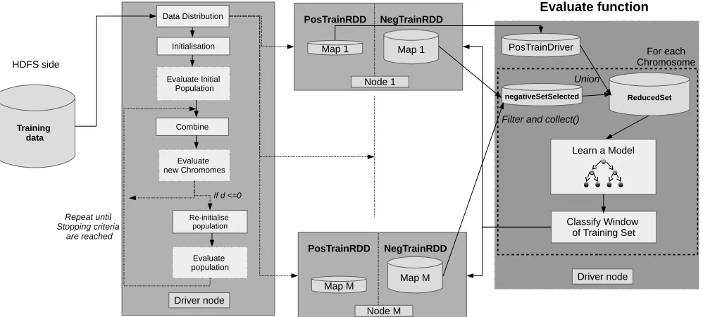
Let trainFile be the training set stored in the HDFS as a single file. This file is composed ofhHDFS blocks that can be examined from any computing node. The global EUS al-gorithm starts off reading the entiretrainFileset from HDFS as an RDD, splitting the dataset into an user-defined number of #Map disjoint partitions (Instruction 1). This operation spreads the data across the computing nodes, caching the different subsets (Map₁,Map₂,...,Mapm) into main memory. Using a function toLabeledPoint(), the original text data is transformed into the LabeledPoint data structure of Spark.

Next, we split this dataset into two subsets: positive set posTrainRDDand negative setnegTrainRDD, which contain only positive and negative instances, respectively. The filter transformation provided by Spark is used for this purpose. For sake of simplicity on the implementation of the chromo-somes, the negative training set is zipped with indexes (using zipWithIndex() operation, see Instruction 2). In this work, we assume that the number of existing positive instances is so reduced that it will perfectly fit in the main memory of the driver node (as we did in [16]. Thus, Instruction 3 also collects the data from worker nodes and bring it to the driver. We will use this copy of the positive training set posTrainDriver later on.

When the data is well distributed across the cluster of com-puting nodes, we can now create the initial population and assess its quality (Instructions 5-8). To do so, we first follow the scheme explained above, creating sparse chromosomes at random. Later, we have to evaluate the quality of such chromosomes.

Algorithm 2 deepens into the necessary instructions to carry out such relevant operation. For each chromosome we have a collection of indexes representing the instances selected from the negative training set. On the one hand, we have to obtain the actual subset of the training set that is represented by the indexes of every chromosome of the population (from now on reducedSet). On the other hand, we have to evaluate such a subset against the training set.

To obtain the actual subset of the training set, we first have to filter the negative training set according to the indexes contained in the current chromosome. To do this, once again, we rely on the filter function provided with Spark (Instruction 2 of Algorithm 2). Since this is going to be a fairly small dataset, we also collect the data from the worker nodes to the driver. Next, both the selected negative instances and all the local copy of positive instances (posTrainDriver) are joined together (Instruction 3 of Algorithm 2) to form the resulting reducedSet.

Typically, the nearest neighbour algorithm is used to classify the training set withreducedSet. Due to the way of working of nearest neighbor, this would oblige us to have the reducedSetavailable in every single node (using for example the broadcast function). However, after some preliminary experiments with this approach, we concluded that the

over-head created sending such information from the driver to the nodes slows down quite a lot the fitness function evaluation, compromising the feasibility of the whole approach.

For this reason, we base the fitness function on an eager model (specifically a Decision Tree), so that, we can learn a single model in the driver node, and broadcast it over all the worker nodes to classify the training set (See Instructions 4-5 in Algorithm 2). The main benefit of doing this is that the model will be a very small data structure compared to the reducedSet, and the classification phase will also be faster than in the case of nearest neighbour.

To accelerate the fitness evaluation, we are based on the windowing scheme defined in [15]. Under such scheme, the chromosomes will only be assessed against a subset of the training set each evaluation. It always includes the entire positive set and a random subset of the negative training set. Both datasets (posTrainRDD and negTrainRDD) were formerly in the form distributed datasets. Therefore, applying transformations on them is very straighforward and not very time consuming operations. Specifically, we randomly take negative instances according to the a given number of windows (established in [15] as the imbalanced ratio). Later, this the entire positive set is joined using theunionoperation, obtaining the window of the training set used for fitness evaluation. The detailed operation can be found in Instruction 6 of Algorithm 2.

After that, the classification takes place. We make use of a mapPartitions(func)transformation to concurrently access to the instances contained in the windowset. The function to be applied in every single portion of the data consists of classifying every single instance using the model broad-cast before. As a result, this function will provide pairs

< trueclass, predictedclass > for each instance of the window. This information is brought to the driver node to compute the g-mean as fitness measure.

When the initial population is evaluated, this is sorted according to their fitness values (Instruction 10). Then, the CHC algorithm enters into a loop (Instructions 11 to 29) where search relies upon recombination and repro-duction to create new potential solutions until a number of evaluation (M AX EV ALU AT ION S) is reached or we have re-initialised the population a number of times (M AX REIN IT IALISAT ION S). This loop includes all the operations described before about the evolutionary pro-cess i.e. crossover with incest prevention (Instructions 12-15), elitist selection (Instructions 20-21), and reinitialisation of the population (Instructions 23-27).

As a result of the evolutionary process, we will obtain a balanced reduced set of instances that globally represent the entire training set. This dataset will be later used by a classifier to learn a model and classify the test set. In particular, we will use the Decision Tree provided in Apache Spark to classify the test set.

Fig. 3: EUS-global: Data flow

Algorithm 1 EUS Global preprocessing Require: trainFile; #Maps; #Windows

1:trainRDD←textFile(trainFile, #Maps).toLabeledPoint().cache()

2:negTrainRDD = trainRDD.filter(line→line.contains(”negative”)).zipWithIndex()

3:posTrainRDD = trainRDD.filter(line→line.contains(”positive”))

4:posTrainDriver = posTrainRDD.collect()

5:d = L/2

{Initialisation}

6:fori= 1toNP do

7: populationi= Randomly take numPositive indexes in the range [0,M-1].

8: fitnessi = evaluate(populationi, negTrainRDD, posTrain-Driver,#Windows )

9:end for 10: population.sorted

11: while eval < MAX EVALUATIONS and reinitialisations < MAX REINITIALISATIONS do

12: offspring = combine(population)

13: ifoffspring.size >0then

14: evaluate(offspring,negTrainRDD, posTrainDriver,#Windows)

15: offspring.sorted

16: end if

17: if offspring.size == 0 or offspring(0).fitness <

population(0).fitnessthen

18: d = d - 1

19: else

20: population = (offspring ++ population).sorted.take(NP)

21: evaluate(population.tail,negTrainRDD, posTrainDriver,#Windows)

22: end if 23: ifd<=0then 24: diverge(population)

25: d = L/2

26: reinitialisations += 1

27: end if 28: end while

IV. PRELIMINARY RESULTS AND DISCUSSION

In order to assess the proposed method for imbalanced big data, we have conducted some preliminary experiments in one big dataset. It comes from the Evolutionary Big Data Competition ECBDL’14 [24], [25]. For this study, we consider a subset of 10% of the instances, in which the number of features was reduced from 631 to 90 by means of the feature selection algorithm applied in [25]. This dataset contains a total of 3,489,083 instances, from which 69,133

Algorithm 2 EUS-global: Parallel fitness function using Spark

Require: population; negTrainRDD; posTrainDriver; NumWindows

1:fori= 1toNP do

2: negativeSetSelected = negTrainRDD.filter{case (key, value) → popula-tion(i).contains(key).collect()}

3: reducedSet = negativeSetSelected.union(posTrainRDD)

4: model = LearnDecisionTree(reducedSet)

5: model broadcast sc.broadcast(model)

6: window = negTrainRDD.mapPartitions(dataset → RandomSelec-tion(NumWindows)).union(posTrainRDD)

7: Outputs = window.mapPartitions(dataset → Classify(dataset, model broadcast)).collect()

8:end for

9:return ComputeGmean(Outputs(True Class, Predicted Class))

belong to the positive class (i.e. an imbalanced ratio of 49, approximately).

In our experiments we consider a 5-fold stratified cross-validation model, meaning that we construct 5 random par-titions of each dataset maintaining the prior probabilities of each class. Each fold, corresponding to 20% of the data is used once as test set, evaluated on a model trained on the combination of the 4 remaining folds. The reported results are taken as averages of the five partitions. To evaluate our model, we consider the AUC and g-mean measures recalled in Section II-B.

The experiments have been carried out on twelve nodes in a cluster: a master node and eleven computing nodes. Each one of these computing nodes has 2 Intel Xeon CPU E5-2620 processors, 6 cores per processor (12 threads), 2.0 GHz and 64GB of RAM. The network is Gigabit ethernet (1Gbps). In terms of software, we have used the Cloudera’s open-source Apache Hadoop distribution (Hadoop 2.6.0-cdh5.4.2) and Spark 1.6.2. A maximum of 216 concurrent tasks are available.

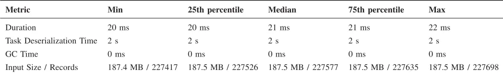
TABLE I: A snapshot of Apache Spark web UI when running collection of the negative selected set (Instruction 2 fro Algorithm 2. It illustrates the main bottleneck we experience in the current implementation of our proposal

Metric Min 25th percentile Median 75th percentile Max

Duration 20 ms 20 ms 21 ms 21 ms 22 ms

Task Deserialization Time 2 s 2 s 2 s 2 s 2 s

GC Time 0 ms 0 ms 0 ms 0 ms 0 ms

Input Size / Records 187.4 MB / 227417 187.5 MB / 227526 187.5 MB / 227577 187.5 MB / 227635 187.5 MB / 227698

V. CONCLUDING REMARKS

In this contribution we have carried out a first attempt on global evolutionary undersampling for imbalanced big data classification. To do so, we have been focused on Apache Spark as big data technology. The main advantage of this model in comparison to existing local approaches is that it will analyse all the data as a whole. Our preliminary results show the potential of this scheme. However, we still need to resolve some technological issues to make sure that the evaluation of the fitness function is fast enough. As future work, we consider that the design of hybrid approaches that accelerate even more the fitness function evolution may result in a very suitable approach to deal with imbalance big data classification from a global perspective.

REFERENCES

[1] M. Minelli, M. Chambers, and A. Dhiraj, Big Data, Big Analytics: Emerging Business Intelligence and Analytic Trends for Today’s Busi-nesses (Wiley CIO), 1st ed. Wiley Publishing, 2013.

[2] M. Zaharia, M. Chowdhury, T. Das, A. Dave, J. Ma, M. McCauley, M. J. Franklin, S. Shenker, and I. Stoica, “Resilient distributed datasets: A fault-tolerant abstraction for in-memory cluster comput-ing,” inProceedings of the 9th USENIX conference on Networked Systems Design and Implementation. USENIX Association, 2012, pp. 1–14.

[3] S. Ghemawat, H. Gobioff, and S.-T. Leung, “The google file system,” in Proceedings of the nineteenth ACM symposium on Operating systems principles, ser. SOSP ’03, 2003, pp. 29–43.

[4] J. Dean and S. Ghemawat, “Mapreduce: simplified data processing on large clusters,”Communications of the ACM, vol. 51, no. 1, pp. 107–113, Jan. 2008.

[5] A. Fern´andez, S. R´ıo, V. L ´opez, A. Bawakid, M. del Jesus, J. Ben´ıtez, and F. Herrera, “Big data with cloud computing: An insight on the computing environment, mapreduce and programming frameworks,” WIREs Data Mining and Knowledge Discovery, vol. 4, no. 5, pp. 380– 409, 2014.

[6] K. Grolinger, M. Hayes, W. Higashino, A. L’Heureux, D. Allison, and M. Capretz, “Challenges for mapreduce in big data,” inServices (SERVICES), 2014 IEEE World Congress on, June 2014, pp. 182–189. [7] A. F. Project, “Apache flink,” 2017. [Online]. Available: https:

//flink.apache.org/

[8] I. Triguero, D. Peralta, J. Bacardit, S. Garc´ıa, and F. Herrera, “MRPR: A mapreduce solution for prototype reduction in big data classifica-tion,”Neurocomputing, vol. 150, pp. 331–345, 2015.

[9] J. Maillo, S. Ram´ırez, I. Triguero, and F. Herrera, “knn-is: An iterative spark-based design of the k-nearest neighbors classifier for big data,” Knowledge-Based Systems, vol. 117, pp. 3 – 15, 2017, volume, Variety and Velocity in Data Science.

[10] V. L ´opez, A. Fern´andez, S. Garc´ıa, V. Palade, and F. Herrera, “An insight into classification with imbalanced data: Empirical results and current trends on using data intrinsic characteristics,” Information Sciences, vol. 250, no. 0, pp. 113 – 141, 2013.

[11] G. Weiss, “Mining with rare cases,” inData Mining and Knowledge Discovery Handbook. Springer, 2005, pp. 765–776.

[12] M. Galar, A. Fern´andez, E. Barrenechea, H. Bustince, and F. Herrera, “A review on ensembles for the class imbalance problem: Bagging-, boosting-Bagging-, and hybrid-based approachesBagging-,” IEEE Transactions on Systems, Man, and Cybernetics, Part C: Applications and Reviews, vol. 42, no. 4, pp. 463–484, 2012.

[13] M. Galar, A. Fern´andez, E. Barrenechea, and F. Herrera, “Eusboost: Enhancing ensembles for highly imbalanced data-sets by evolutionary undersampling,”Pattern Recognition, vol. 46, no. 12, pp. 3460–3471, 2013.

[14] S. Garc´ıa and F. Herrera, “Evolutionary under-sampling for classifica-tion with imbalanced data sets: Proposals and taxonomy,”Evolutionary Computation, vol. 17, no. 3, pp. 275–306, 2009.

[15] I. Triguero, M. Galar, S. Vluymans, C. Cornelis, H. Bustince, F. Her-rera, and Y. Saeys, “Evolutionary undersampling for imbalanced big data classification,” inEvolutionary Computation (CEC), 2015 IEEE Congress on, May 2015, pp. 715–722.

[16] I. Triguero, M. Galar, D. Merino, J. Maillo, H. Bustince, and F. Herrera, “Evolutionary undersampling for extremely imbalanced big data classification under apache spark,” in2016 IEEE Congress on Evolutionary Computation (CEC), July 2016, pp. 640–647. [17] L. J. Eshelman, “The CHC adaptive search algorithm: How to have

safe search when engaging in nontraditional genetic recombination,” inFoundations of Genetic Algorithms, G. J. E. Rawlins, Ed. San Francisco, CA: Morgan Kaufmann, 1991, pp. 265–283.

[18] A. H. Project, “Apache hadoop,” 2013. [Online]. Available: http://hadoop.apache.org/

[19] T. Fawcett, “An introduction to roc analysis,” Pattern recognition letters, vol. 27, no. 8, pp. 861–874, 2006.

[20] S. del R´ıo, V. L ´opez, J. Ben´ıtez, and F. Herrera, “On the use of mapreduce for imbalanced big data using random forest,”Information Sciences, vol. 285, pp. 112–137, 2014.

[21] L. Breiman, “Random forests,”Machine learning, vol. 45, no. 1, pp. 5–32, 2001.

[22] V. L ´opez, S. del R´ıo, J. Ben´ıtez, and F. Herrera, “Cost-sensitive linguistic fuzzy rule based classification systems under the mapreduce framework for imbalanced big data,”Fuzzy Sets and Systems, vol. 258, pp. 5–38, 2014.

[23] S. Garc´ıa, J. Derrac, J. Cano, and F. Herrera, “Prototype selection for nearest neighbor classification: Taxonomy and empirical study,”IEEE Transactions on Pattern Analysis and Machine Intelligence, vol. 34, no. 3, pp. 417–435, 2012.

[24] “ECBDL14 dataset: Protein structure prediction and contact map for the ECBDL2014 big data competition,” 2014. [Online]. Available: http://cruncher.ncl.ac.uk/bdcomp/