Journal: New Phytologist Article type: Modeling /Theory
OpenSimRoot
: Widening the scope and application of root architectural models
Postma, Johannes A.1, Kuppe, Christian1 , Owen, Markus R.2,3, Mellor, Nathan3,4, Griffiths, Marcus3,4, Bennett, Malcolm J.3,4, Lynch Jonathan P.3,4,5, Watt, Michelle 1
1) Plant Sciences, Institute of Bio and Geosciences 2, Forschungszentrum Jülich, Wilhelm-Johnen Straße 52425 Jülich, Germany
2) Centre for Mathematical Medicine and Biology, School of Mathematical Sciences, University of Nottingham, Nottingham, NG7 2RD, UK
3) Centre for Plant Integrative Biology, University of Nottingham, Nottingham, LE12 5RD, UK 4) Plant & Crop Sciences Division, School of Biosciences, University of Nottingham, Nottingham, LE12 5RD, UK
5) Department of Plant Science, Pennsylvania State University, 102 Tyson Building, University Park, PA 16802, USA
Author for correspondence: Johannes A. Postma, email: [email protected], telephone: +49(0)2461614333, twitter: @j_a_postma
Total word count: (regular research papers should not exceed 6500 words): Currently 6254 Word count Summary: 193
Word count Introduction: 669 Word count Description 3866 Word count Results 1075 Word count Discussion 451
Word count Acknowledgements & Author contributions: 217 Number of Figures: 6
1
2
3 4
5 6
7
8 9
10 11
12
13 14
15 16
17
18 19
20
21
22
23
24
25
26
27
Summary
Research Conducted and Rationale: OpenSimRoot is an open sourced, functional-structural plant model and mathematical description of root growth and function. We describe OpenSimRoot and its functionality to broaden the benefits of root modeling to the plant science community.
Description: OpenSimRoot is an extended version of SimRoot, established to simulate root system architecture, nutrient acquisition, and plant growth. OpenSimRoot has a plugin, modular infrastructure, coupling single plant and crop stands to soil nutrient, and water transport models. It estimates the value of root traits for water and nutrient acquisition in environments and plant species.
Key results and unique features: The flexible OpenSimRoot design allows upscaling from root anatomy to plant community to estimate 1) resource costs of developmental and
anatomical traits, 2) trait synergisms, 3) (inter species) root competition. OpenSimRoot can model 3D images from MRI and X-ray CT of roots in soil. New modules include: 1) soil water dependent water uptake and xylem flow, 2) tiller formation, 3) evapotranspiration, 4) simultaneous simulation of mobile solutes, 5) mesh refinement, and 6) root growth
plasticity.
Conclusion: OpenSimRoot integrates plant phenotypic data with environmental metadata to support experimental designs and gain mechanistic understanding at system scales.
Keywords: Root system architecture, Functional Structural Plant Model, OpenSimRoot, Root architectural traits, Simulation, Model driven Phenotyping, Plant nutrition
30
31
32 33 34
35
36 37 38 39
40
41 42 43 44 45 46
47
48
49
50 51 52
Introduction
Functional-structural plant models combine a representation of 3D plant structure with
physiological functions to advance plant science and its applications (Vos et al., 2010; Dunbabin et al., 2013). Those that incorporate below-ground root parameters (Dunbabin et al., 2002; Pagès et al., 2004; Wu et al., 2007; Pierret et al., 2007; Javaux et al., 2008; Leitner et al., 2010; Lobet et al., 2014; Gérard et al., 2017), require significant time and expertise in biological, mathematical, computational and digital image analyses, and therefore their development benefits greatly from an open and global setting. SimRoot is one of the most feature-rich and highly cited
functional-structural root architectural models. However the last full description dates back twenty years (Lynch et al., 1997), and subsequent papers report application of the model, with successive changes embedded in methods sections (Postma & Lynch, 2011a,b; Dathe et al., 2013). Here we describe fully a new, open source version, branded OpenSimRoot, that is freely available for
download (http://rootmodels.gitlab.io/ OpenSimRoot). New features in this version allow simulation of more growth scenarios and crops, and its application has been widened to support emerging root phenotyping technologies.
SimRoot was originally designed to reconstruct root system architecture (RSA, see Table 1) from
empirical data such as growth rates, angles and branching frequencies of different root classes. A post-simulation analysis of root geometry, nutrient uptake, and carbon costs enabled comparison of different RSAs with respect to their efficiency in taking up phosphorus relative to carbon costs (Nielsen et al., 1994; Lynch & Beebe, 1995; Nielsen et al., 1997; Lynch et al., 1997; Ge et al., 2000; Rubio et al., 2001; Walk et al., 2004, 2006). Later versions coupled physiological
mechanisms such as root respiration, nutrient uptake, canopy photosynthesis, and RSA to simulate how the root phenotype dynamically interacts with the soil environment, and how this interaction influences acquisition of soil resources and consequently plant growth (Postma & Lynch, 2011a,b, 2012; Dathe et al., 2013; Postma et al., 2014a; Dathe et al., 2016; York et al., 2016). The initial focus was on phosphorus capture (Lynch & Beebe, 1995; Ge et al., 2000; Ma et al., 2001; Postma & Lynch, 2011b), which was later expanded to include C (photosynthesis), N, K, and water (Postma
et al., 2008; Postma & Lynch, 2011a; Dathe et al., 2013). Microeconomic theory, in which resource
acquisition is compared to resource investment costs, has guided the interpretation of results (Lynch, 2007; Postma et al., 2014b). Although SimRoot was designed as a heuristic model, i.e., a tool for exploring implications of existing knowledge, and gaps in that knowledge, it proved surprisingly accurate for predicting fitness outcomes of root phenotypes (Chen et al., 2011; Saengwilai et al., 2014; Zhan et al., 2015).
SimRoot is one of several root models that have been developed. Dunbabin et al. (2013) presents an exhaustive review of all root models to date and their capabilities. To our knowledge OpenSimRoot
is currently the only plant root model that is openly version controlled (GIT) and GPLv3 licensed, allowing community-driven development. We envision that OpenSimRoot will be used and
expanded by both modelers and non-modelers to simulate RSA and nutrient and water uptake in an ever widening scenario for species, environments and crop management practices to advance root-based opportunities to increase resource-efficient agricultural productivity. A design goal of
OpenSimRoot is a flexible model structure that can be controlled by the user rather than the
programmer. This means that, through a plugin infrastructure, the user can directly vary components of the model and compare the results. Model behavior can further be studied through sensitivity analysis, which has been a major focus in past publications.
In this paper we initially provide a short description of the design of the OpenSimRoot model and definitions, then present the major submodels in OpenSimRoot which simulate RSA, the shoot, carbon, water and nutrient acquisition and utilization, root growth plasticity, and geometric descriptors. After this model description we discuss model implementation, which is designed for flexibility, extensibility, transparency and robust numerics. We conclude with several examples of
OpenSimRoot usage.
Model description
OpenSimRoot has, compared to other root models, a unique design which centers on coupling
various mini-models (For definitions see Table 1). The distinction between parameter and algorithm has been, in line with object oriented programming, removed by encapsulating both within classes which share a common interface for coupling and data exchange.
OpenSimRoot design
OpenSimRoot contains a command line interface (CLI), a simulation engine, a plugin library, and
classes responsible for reading and writing of data (Figure 1, Notes S1,2,3&4). The simulation engine implements an application programming interface (API) through which different modules can request information (See Note S1). The plugin infrastructure allows developers to implement new modules with limited knowledge about the rest of the code. Each plugin establishes
dependencies between minimodels through the API and requests data of other minimodels in order to compute the necessary information. At the start of execution the import module reads an XML file (see below) and, based on that file, constructs a tree of minimodels. According to the
specification in the XML, the minimodels load (instantiate) appropriate algorithms from a registry 87
88 89 90 91 92 93 94 95 96 97
98 99 100 101 102 103
104
105 106 107 108
109
which lists all available plugins (Note S3). The plugin infrastructure not only allows the user to implement new processes, but also to implement alternative algorithms and compare model results. The behavior of the modules described below is thus not fixed but can be adapted to hypotheses. Simulation is driven based on data requests that originate from the users request for output. Upon instantiation of the object tree, the modules that write output start requesting information in order to write the output files. The CLI has a small number of options (listed with –h) with the most
important one the input file name. Runs are non-interactive such that many runs with different parameter combinations can be fully automated on a computational cluster. This capability is important when large numbers of simulations are required, for example when exploring parameter sensitivity or processing real root structures (see Results) from large numbers of plants.
Description of the various modules
Root growth and RSA. The root system is represented by vertices and edges in OpenSimRoot. Every root tip has its own vertex with dynamic coordinates, and all other vertices have stationary coordinates that are placed behind the root tip as it extends. The final discretization of the root system can be coarser than the frequency of each growth point’s directional change. A fine scale discretization request can automatically reduce the integration time step. In the case of a coarse discretization, the length of a root segment is not the linear distance between two vertices, but the true distance that the root grew, based on growth rate at that given time. We thus “simplify” the growth trajectory for computational reasons, without losing the true root length.
To grow a root system, we need: 1) when and where root tips (primordia) are created, 2) how fast root tips grow, and 3) in what direction. To start, we assume that, at a minimum, one primary root and a hypocotyl are present in the seed embryo. The term hypocotyl is used here freely to include any shoot axiles (stems) that are the origins of adventitious roots, whether simulating dicotyledons or monocotyledons. Branch roots and their own branch roots (classed according to order), are assumed to emerge from the primary root, based on rules that control the timing and placing of the branches. Adventitious roots (crown or nodal roots in grasses) can branch from the stem according to different schemes; the simplest defined by a starting time and position of a single whorl of roots. Formation of branch roots from these axiles is typically based on branching frequencies, which can be expressed in time, or space, or both, where the missing information is computed based on the growth rate of the parent root. Roots can branch from either phloem or xylem poles, depending on species (Casimiro et al., 2003). The number of poles determines number of positions of the radial branching angle, while the axial branching angle (angle between parent root and branch) is given in the parameter section (for detailed explanation see Lynch, 1997, and Figure 2).
Elongation rates of individual roots are predefined in the parameter space, but might be scaled according to a “root vigor” scaling factor; for example drawn from a lognormal distribution of elongation rates (scaled to unity), thus creating variation in length. The vigor factor can also scale the root specific root diameter, to allow an allometric relation between elongation rate and root diameter expansion within a root class (Pagès, 2000; Wu et al., 2016). Initial root diameter is otherwise a root class specific input parameter.
While initial growth direction is set by specified radial and axial branching angles (Figure 2), the direction can be changed with a tropism vector. The tropism vector is the sum of several vectors representing gravitropism, random impedance, and nutrient tropisms and is added to the normalized growth direction vector, to obtain the new direction.
Once the root is growing, its branching rules allow it to branch off new roots of different classes and the whole process is repeated. Although OpenSimRoot currently does not simulate shoot
architecture, a simple tiller model is included. Tillers can form their own leaf area, and their own root systems. In grasses, tillers produce nodal roots which can form a significant fraction of the total root system, depending on species and environment (Atkinson et al., 2014; Sebastian et al., 2016). Tiller formation is done on the basis of a table that indicates the time dependent delay till the next tiller is formed. Dicotolydonous roots have secondary growth from cambia which thicken the stele and periderm in the root. Secondary growth is simulated using a time dependent radial growth rate, scaled to distance along the root.
Simulation of shoot growth and related processes. A simple shoot model can be constructed with
OpenSimRoot plugins. The shoot model is non-geometric and represents the shoot by the state
variables leaf area and leaf and stem dry weight. Increase in dry weights is based on carbon
intercepted light is converted linearly to carbon fixation. Intercepted light is computed from leaf area index, assuming that the simulated plant is in a homogeneous canopy of equally spaced and identical plants. Tillers are simulated as new plants with their own leaf area, but sharing resources. Carbon allocation to roots. The root growth module can compute the carbon for growth for each root segment (edge) using its volumetric increase, and a specific root volume (g cm-3). Volume increases arise from primary and/or secondary growth, and root segments are assumed cylindrical or, in the case of varying diameters, a truncated cone. OpenSimRoot compares available to required carbon, and if source strength is greater than sink strength, stores the carbon left over into a labile pool. OpenSimRoot thus considers that plant growth may be physiologically, not resource,
constrained (Postma et al., 2014b). The labile pool is depleted when sink strength (defined by carbon needed for potential growth) is greater than source strength. Once stored carbon is depleted, growth rates decline. Various rules for carbon allocation under source limiting conditions have been implemented. The most used rule to date prioritizes shoot over roots, and within the root system, secondary growth (root cambial thickening) over elongation, and within the root classes, elongation of major bearing roots over branch roots. Consequently, when plant growth is carbon limited, growth rates of branch roots are reduced more than the growth of the parent roots. These rules do not have a physiological basis, rather a pragmatic basis in which source sink imbalances are seen as errors in the parameterization and estimation of the growth rates, and the assumption is that these errors are more likely in the branch root growth than in the shoot growth. However, other rules, such as equal scaling of all organs have been implemented, and can be used if the user assumes that all sinks compete equally for the available carbon.
Although the inputs of the model are absolute growth rates, allometric scaling, based on the ratio between actual and potential leaf area (not mass), can reduce the attainable growth rate of the canopy and the rate of formation of new root branches. This implies that plants can never fully recover from a stress. However, a recovery rate can be defined which allows the plant to grow, for example, 10% faster when resources permit. Allometric scaling can also be used for the formation of branches. For example, the number of nodal roots per whorl in maize is dependent on the size of the shoot.
Hydrology. OpenSimRoot includes a hydrology module (Figure 3). The implementation of the hydrology module involves the coupling of three models that simulate the movement of water through soil, plant and into the atmosphere. OpenSimRoot includes a simplified C++
evapotranspiration is simulated using the Penman-Monteith equation (Penman, 1948; Monteith, 1964). Small adjustments of these models, to achieve good coupling, are described in Note S5. The hydrology module provides 3D water uptake profiles, drives convective nutrient transport, and can simulate compensatory water uptake and hydraulic redistribution, which may occur when the top soil dries out, causing nutrient uptake from dry soil domains to be reduced. It currently does not simulate drought related growth responses.
Nutrients. OpenSimRoot has a nutrient module to simulate the simultaneous uptake of solutes, originally implemented to simulate the impact of RSA on nutrient uptake, and to test tradeoffs for acquisition of nutrients (Postma & Lynch, 2011a; Dathe et al., 2013). Postma et al. (2014a) showed how the optimal branching density in maize depends on the relative availability of phosphorus and nitrogen. The module involves three parts: 1) simulation of plant nutrient requirements, 2)
simulation of nutrient acquisition, and 3) stressors which define how suboptimal plant nutrient concentrations affect physiology or growth (Figure 4). Nutrients are simulated independently of each other, except that in step (3) the impact of suboptimal nutrient concentrations on a given state variable is aggregated using a maximum or averaging function. For example, nitrogen might affect photosynthesis more than phosphorus, but phosphorus might affect the leaf area expansion rate more strongly (see Dathe et al., 2013).
The nutrient requirements of the plant are determined by integrating over the whole plant biomass predefined optimal and minimal nutrient concentrations. The plant acquires nutrients through seed reserves, uptake by the root system, and optional nitrogen fixation. Uptake of nutrients by the root system is simulated by Michaelis-Menten kinetics, where movement of nutrients in the soil towards roots is simulated through convection-dispersion-diffusion equations. OpenSimRoot includes two different implementations for solving these equations: 1) The Barber-Cushman model (Itoh & Barber, 1983), which simulates depletion zones around individual root segments at high resolution, and is suitable for immobile nutrients like phosphorus; and 2) a reimplementation of the solute model included in SWMS3D (Šimunek et al., 1995), which couples to the soil water model within the hydrology module (above), simulates the whole soil domain and is suitable for mobile nutrients like nitrate. More detailed descriptions of these models are given in Note S5.
equilibrium might not be reached (Postma & Lynch, 2011b; Postma et al., 2014b). The current implementation assumes that, internally, reallocation of nutrients is fast and perfect, such that all organs experience equal stress. This might be true for a nutrient like nitrogen, which typically causes chlorosis everywhere in the shoot, but might not be correct for other nutrients. The
importance of simulation of nutrient redistribution in the plant still needs study, and would require implementation of a shoot architectural model in which the age and position of individual leaves or canopy strata are simulated.
Mineralization and rhizosphere processes. OpenSimRoot implements the Yang and Janssen model for mineralization (Yang & Janssen, 2000). This model assumes exponential decline of a carbon pool, via aging and decline in break down rate. Based on C/N ratios of the substrate and C/N ratios of the microbial biomass, the net mineralization or immobilization of N can be computed.
OpenSimRoot assumes that ammonium is readily converted to nitrate, and soil water content and
temperature are currently ignored. The implementation of the Yang and Janssen model in
OpenSimRoot simulates mineralization for every FEM node independently and thus mineralization
rates may vary in space. The user can define a nitrogen fixation rate as a percentage of the nitrogen requirements of the plant. Fixation will not directly reduce nitrogen uptake from soil, but improves plant nitrogen status.
Root exudation is not explicitly simulated, but is instead described as a root class- and time-dependent carbon cost. Furthermore, exudation may increase the soluble nutrient concentration in the soil at the cost of the insoluble fraction and thereby increase nutrient availability locally (Barber-Cushman model only).
Root growth plasticity. OpenSimRoot can define reaction curves to local environmental factors, to simulate a localized growth behavior of roots (Figure 5), often termed “plasticity” (Bradshaw, 1965; Palmer et al., 2001). 3D interpolation of available environmental data is used to define values at the root surface. For example, a reaction curve (norm, (Pigliucci et al., 1996)) could describe how gravitropism is scaled according to the local concentration of a nutrient. Similarly, branching frequency or root elongation rates can be scaled according to a local soil variable. For example, static fields for soil compaction can be defined in three dimensions, using lists of coordinates and associated values in conjunction with a spatial interpolation algorithm. Root elongation can then be defined as a function of local soil compaction.
gradients is unclear, and currently no such mechanism has been implemented. OpenSimRoot does, however, include a mechanism to scale the strength of the local plasticity response on the basis of yet another reaction norm which might couple plasticity to whole plant status.
Root length distribution and virtual coring. OpenSimRoot can compute several geometric metrics, specifically root length density profiles, virtual coring, root length below D90 for nitrate, and overlap of depletion zones. Others, like explored soil volume, or fractal dimensions, can be computed by the user on the basis of the geometric model output.
Root anatomy. Root anatomy is not simulated in 3D explicitly, but OpenSimRoot can represent the stele diameter, thickness of the cortex, the degree of cortical senescence, the degree of root cortical aerenchyma formation, and the length, diameter and density of root hairs. These anatomical traits may influence processes at the root segment level, specifically nutrient content, respiration, nutrient uptake and hydraulic conductivity (Fan et al., 2003; Hu et al., 2014).
Implementation
OpenSimRoot is written in C++, an object oriented programming language. OpenSimRoot couples
minimodels, which encapsulate the simulation of a single state variable. State variables are assumed to be associated with time and space and always have a unit. Minimodels are implemented as single C++ classes which inherit from the same base class (named SimulaBase), such that they all have the same interface (API). This interface allows minimodels to connect to other minimodels and request data. Minimodels might encapsulate a constant, an interpolation table, a random number generator or may make use of helper functions for computation. These helper functions are of the class type IntegrationBase and DerivativeBase and are registered under their specific names, such that, based on the input, the correct helper function can be instantiated. Helper functions compute a variable, and when associated with an integration function, can be integrated over time. The true
functionality of OpenSimRoot is thus dispatched to the helper functions. Through a plugin
framework, developers can add new helper functions and thus extend the functionality of the model. Example code for a plugin is given in Note S4.
Thus, coupling of the state variables is done through a simple common interface guaranteeing that minimodels are, from a programmer point of view, standalone objects. Computations are quite indifferent as to how dependent variables are computed. This creates high flexibility in the input files, where the state variables can be defined in a variety of ways, i.e. constant, stochastic, interpolation table, or based on a plugin (Table 2, Note S6).
288 289 290
291 292 293 294
295 296 297 298 299
300
301 302 303 304 305 306 307 308 309 310 311 312 313
One big challenge in coupling independent (mini)models is the implementation of numerical integration when different models have different time steps, and when implicit coupling is desired.
In OpenSimRoot we implemented a general framework for predictor corrected methods, by default
RungeKutta4, with three components: 1) Interpolation, 2) Prediction, and 3) Dependency tracking. Each minimodel keeps a time table to interpolate between time steps and return historical
information. Different minimodels can run at different time steps, which are however synchronized at every globally defined maximum time step. Since all data requests loop through the SimulaBase API, OpenSimRoot tracks forward dependencies and predictions, to determine whether to keep the step taken. Interdependent minimodels (For an exemplar graph of dependencies see Note S7) update using a predictor corrector method with interpolation to ensure compatibility of time steps. Whilst the precise order may have some influence on numerical accuracy or efficiency, there is typically no rational basis on which to prefer any one order of evaluation and is therefore simply dependent on the order of information requests (Typically breadth-first search, see hierarchical contextualization). The independent minimodel approach can create a significant computational overhead. However, simulations of RSA are still relatively fast compared to soil and we regard the ease with which new functionality can be added with no or little programming effort or knowledge about the rest of the code as more important than runtime.
The current implementation of OpenSimRoot only depends on the standard C++ libraries (ISO C+ +11, and a few system libraries for the CLI), and on our website (rootmodels.gitlab.io) we provide directions for compilation and running on Linux, Mac and Windows operating systems.
Hierachical contextualization. Many dynamic models are structured along a sequence of events; the 'time loop'. However, OpenSimRoot represents the plant as a hierarchy of interacting
components to allow the main purpose of understanding of the function of root traits for the whole plant. Minimodels are placed in a simple hierarchy which provides them context, while the object oriented paradigm “hides” the internal workings of each component.
Dynamic adding of components. OpenSimRoot adds (instantiates) new components during simulation to represent newly grown roots. This contrasts with crop models that represent plant growth by an increase in values of the state variables. Dynamic memory management, connected to an object oriented programming paradigm, is a useful programming feature for adding new
by copying templates, which contain all the necessary minimodels that are defined in the input files. An example of an ObjectGenerator plugin is given in Note S4.
Input files
OpenSimRoot uses a hierarchical file of parameter values, which not only contains parameter
values, but all state variables, and their metadata, such as names and units. Hierarchy provides context, such that parameter lists can be specific for different root classes of different plant species. Input files are implemented in XML, a general language for describing data together with metadata that is also hierarchical, flexible, allows comments, is supported by many software tools, and can be rendered in a browser as a more readable document. Note S6 gives an example of an input file that simulates a simple relative growth model.
OpenSimRoot allows the user not only to enter initial values, but arrays of initial time series. This
way, part of the RSA can be predefined, based on measurements (also see examples in Results). This approach may be different from most models, but creates the opportunity to use the model as an extension to phenotyping as partial information derived from phenotypic measurements can be directly entered into the input files (Fiorani & Schurr, 2013, Figure 6). Parameterizations exist for maize, squash, bean, lupin, Arabidopsis, and barley, and are now being developed for wheat and rice (Ma et al., 2001; Chen et al., 2011; Postma & Lynch, 2012). Input files for maize and bean, a predefined root system, a small crop model and other testing scenarios are included in the source code repository (https://gitlab.com/rootmodels/OpenSimRoot).
Output files
OpenSimRoot includes export modules that can be enabled or disabled to retrieve specified output
forms that include tables in text files, 3D models in various VTK (visual tool kit, www.vtk.org) formats, 3D raster images, and a XML formatted dump of the model in the format of
OpenSimRoot’s own input files. For example: tables can be further processed with statistical
software (like R), VTK files can be opened with 3D data viewers (e.g. Paraview,
http://www.paraview.org/), and the model dump can be viewed in a web browser (Note S6).
License
OpenSimRoot is available under the GPLv3 Licence (https://www.gnu.org/licenses/gpl-3.0.en.html)
which is an opensource – copyleft license. The license enables the practice of “good science” by 352
353
354
355 356 357 358 359 360 361
362 363 364 365 366 367 368 369 370
371
372 373 374 375 376 377
378
making the model transparent and by facilitating contributions from a wider range of expertise in the community. Access the version controlled code at https://gitlab.com/rootmodels/OpenSimRoot .
Application examples for
OpenSimRoot
SimRoot has found useful application in several domains, including 1) geometric analysis of root
system form and function, 2) simulation of processes that are very difficult to measure empirically, 3) simulation of dynamic systems, 4) sensitivity analyses, and 5) simulation of hypothetical
systems. In addition, a new capability of OpenSimRoot to read in (partially) predefined RSA enables application as an extension to 3D phenotyping techniques such as X-ray CT (Computed
tomography) and MRI (Magnetic Resonance Imaging). Examples of all of these applications are provided below.
Studies on the function of RSA traits
A primary output of OpenSimRoot is the RSA phenotype emerging from input parameters
simulating specific phenes like gravitropic setpoint angle or lateral root initiation interacting with environmental conditions. For example, due to spatio-temporal heterogeneity in soil nutrient availability, growth angles may differentially affect phosphorus and nitrogen uptake but also affect the degree of inter- versus intra-plant root competition (Ge et al., 2000; Rubio et al., 2001; Dathe et al., 2013). Results of simulated maize-bean-squash intercropping systems showed that RSA and nitrogen fixation (bean) work towards reduced competition and increased biomass (Postma & Lynch, 2012; Zhang et al., 2014). Competition among branches of the same parent root may
become stronger when the root branching density increases, and since this increase results in greater sink strength, but not greater source strength (in carbon available for growth), the individual roots may stay shorter. Simulating these processes, Postma et al. (2014a) estimated that the optimal branching density (assuming parent roots have the same root branching density) for maize was lower when nitrogen availability decreased. The benefit of fewer but longer laterals in low nitrogen soils was confirmed in a genotypic contrast study (Zhan et al., 2015). Walk et al. (Walk et al., 2006) estimated the tradeoffs between basal root growth and adventitious root growth in bean and
concluded that adventitious roots might be of most benefit when phosphorus availability is low. While these RSA traits represent tradeoffs, other traits may work in synergy towards greater productivity on low nutrient soils (Ma et al., 2001; Postma & Lynch, 2011a; Miguel et al., 2015).
OpenSimRoot has also increased understanding of how integrated phenotypes function. This was
demonstrated by York et al.(2015) who used SimRoot to estimate how changes in maize RSA, introduced by breeding over 100 years, might affect the nutrient uptake efficiency of modern 381
382
383
384 385 386 387 388 389 390
391
cultivars. New functionality described here will enable new studies of the function of whole plant traits, such as tiller formation and its influence on RSA.
Relationships between RSA traits and root system descriptors.
Many researchers determine what might be called geometric descriptors of RSA: root length density profiles, fractal geometry, specific root length, total root length, rooting depth and convex-hull (Fitter & Stickland, 1992; Clark et al., 2011). These descriptors can be computed on simulated roots and their relation to architectural, anatomical or functional traits can be inferred. For example, differences in the specific root length of a root system may be related to anatomical changes, or a different ratio of thick to finer roots. Nielsen et al. (1997) determined differences in fractal
dimensions between phosphorus efficient and inefficient genotypes, and Walk et al. (2004) applied
SimRoot to show how soil exploration for P related to the fractal dimensions of the root system.
Miguel et al (2015) applied SimRoot to do “virtual coring” in order to support the idea that genotypic differences in rooting depth might best be seen when coring in between rows. These studies show how the geometric aspects of the root system can be related to root traits and function, something not easily derived from empirical measurements of actual root systems.
Scaling up from root anatomy to crop
At its smallest spatial scale, OpenSimRoot represents root anatomy, and at its largest scale it simulates crop measures like biomass, nutrient uptake and root zone depletion and leaching. For example, Ma et al., (2001) focused on root hairs in Arabidopsis thaliana and concluded that their length and density contribute synergistically towards greater phosphorus uptake. Chen et al., (2011, 2013) used SimRoot and lupin phenotypic data to compute that the contribution of root hairs to total phosphorus uptake might vary strongly among genotypes. Postma and Lynch (2011a,b) and
Schneider et al. (unpublished) simulated the root class- and time-dependent formation of Root Cortical Aerenchyma (RCA) and Root Cortical Senescence (RCS) respectively, and determined that RCA and RCS may be mechanisms underlying greater growth on low nutrient soils in maize, bean and barley, possibly via efficient use and recycling of resources. Genotypic contrast studies on low N soils concur with these simulation results (Saengwilai et al., 2014) which suggests that
OpenSimRoot can be used for scaling up from anatomy to crop stands.
OpenSimRoot as an extension to plant phenotyping
413414
415
416 417 418 419 420 421 422 423 424 425 426 427
428
429 430 431 432 433 434 435 436 437 438 439 440
Technologies like X-ray CT and MRI have been adapted to image root systems non-destructively and provide non-invasive ways to phenotype whole root systems in 3D in soil (Mooney et al., 2012; Mairhofer et al., 2013; van Dusschoten et al., 2016). The utility to feed such data to a model was demonstrated by Stingaciu et al. (2013) for a non-growing lupin root system. Using time estimates,
OpenSimRoot can simulate the growth of a root system such that the RSA is identical to that
imaged. Figures 6a,b (for animation see Movie S1) show an MRI image, and the simulated root system. The simulation does not include a small portion (~8%) of the roots visible in the 3D image data because of limitations in image segmentation, rather than in the model. OpenSimRoot can add “MRI-non-visible” finer roots to the simulation according to existing model rules, and the
simulation can be extended beyond the measured time, to predict continued growth of the root system. Importantly, OpenSimRoot modules for nutrient and water uptake can be enabled with the architectural phenotypes derived from measurements and simulation, and functions can be ascribed to the traits. This may help researchers and breeders go from image to functional understanding of the measured root systems, and compare genotypes not only on the basis of geometry, but also on the basis of modeled ability to take up water and nutrients. For example, Figures 6c,d show a CT image, and corresponding OpenSimRoot simulation of nitrate depletion zones around the root system. Integration of the model into phenotyping pipelines is also likely to help find deficits of the model, and give modelers a basis for improving parameterization and/or algorithms. This important development considerably widens the scope of application of OpenSimRoot.
Discussion & Conclusions
We have described the first open source version of the RSA model SimRoot, which is now available for use by biologists and modelers. New features that expand its use include hydrology to simulate and understand root system hydraulic properties. A novel area of application includes simulation of non-invasive 3D phenotypic data of RSA from MRI and X-ray CT, and their putative functions in nutrient and water uptake. To our knowledge, OpenSimRoot is currently the most feature rich and widely published multiplatform RSA model (Dunbabin et al., 2013) that is freely available for direct download (http://rootmodels.gitlab.io/ OpenSimRoot). The new open-source implementation combines features that will enable expansion of use for plant and crop science:
a modular, plugin infrastructure for extending the model;
a default predictor-corrected numerical scheme for integration and coupling;
the ability to predefine any data that was measured, where the model will use the measured data instead of its algorithm for simulation (e.g. the root system, and optionally its history, may be partly pre-defined based on MRI or CT images);
integration with a shoot model;
ability to simulate competition among plants of different species;
maintained by an international community of root researchers.
Relationships in crop models that are typically only defined empirically, such as competition among roots for nutrients, or root length density profiles, are actually a result of RSA, and therefore, RSA models provide insight into relations between measurable traits and emerging properties at the crop level. We regard the heuristic value of the model, and its use as a tool for developing and testing of concepts, and prediction of mechanisms and trends, as the more important motivation for model studies with, and continued development of, OpenSimRoot. The model may have further utility in extending phenotyping pipelines by estimating genotype performance based on measured root phenotypes.
Future development will be community driven, and may include new processes such as root signaling networks, drought responses, soil microbial interactions and soil chemistry. As our mechanistic understanding of different processes increases, OpenSimRoot’s hierarchical structure allows new empirical data to be represented by new algorithms. For example, gravitropism may be simulated on the basis of understanding of differential cell elongation rather than on the current empirically derived input. Open sourcing allows other modelers to couple OpenSimRoot to their models. For example shoot architectural models might be coupled to OpenSimRoot, in order to understand competition for light and shoot architectural traits in relation to RSA traits. Finally, opening up the code enables developers of other RSA models to compare the results of
OpenSimRoot to those of their models, which may lead to constructive critique and improvements
of all RSA models, and by extension, discoveries for improvements in understanding of plant and crop resource efficiencies.
Acknowledgements
We would like to acknowledge all the researchers who over the past 25 years have contributed to the development of OpenSimRoot, in particular RD Davis, Kai L. Nielsen, Gerardo Rubio,
Zhenyang Ge, Raul Jaramillo, Tom Walk, Annette Dathe, Larry York, Eric Nord, Harini Rangajaran, Vera Hecht, Hannah Schneider and Ernst Schäfer. We would also like to thank Darren Wells and Dagmar van Dusschoten for contributing the CT and MRI images, respectively, and Daniel Pflugfelder for assistance in segmenting and analyzing the MRI image.
This research received support from the Forschungszentrum Jülich in the Helmholtz Association, and the German-Plant-Phenotyping Network that is funded by the German Federal Ministry of 475
476
477
478 479 480 481 482 483 484 485
486 487 488 489 490 491 492 493 494 495 496 497
498
499 500 501 502 503 504
Education and Research (project identification number: 031A053).
Author contributions
J.A.P. and M.W. planned the manuscript. J.P.L. conceived of SimRoot and led its development through 2011, J.A.P. rewrote the code, expanded its capabilities, and has led its development since 2011, with mathematical support from C.K. since 2013. J.A.P., C.K., N.M. and M.R.O. programmed various parts of the model code. All authors were involved in open sourcing of the code and
forming a development team. M.J.B., N.M., M.G. and M.R.O. contributed the CT image data and the simulation output based upon that data. J.A.P., C.K., M.W., J.P.L. M.R.O. and M.J.B. wrote various parts of the manuscript, with input from all authors.
Supplemental files
Note S1: Description of the SimulaBase API
Note S2: How to run OpenSimRoot: description of the comman line interface CLI. Note S3: Overview of all classes that form OpenSimRoot, including list of plugins Note S4: Example C++ code for a plugin
Note S5: Technical description of water and nutrient modules Note S6: Example input file
Note S7: Example graph of state variables and their dependencies Movie S1: Animation of Figure 6.
507
509
510 511 512 513 514 515 516
517
518
519
520
521
522
523
524
References
Alm DM, Cavelier J, Nobel PS. 1992. A finite-element model of radial and axial conductivities for individual roots: development and validation for two desert succulents. Annals of Botany 69: 87–92. Atkinson JA, Rasmussen A, Traini R, Voß U, Sturrock C, Mooney SJ, Wells DM, Bennett MJ. 2014. Branching Out in Roots: Uncovering Form, Function, and Regulation. Plant Physiology 166: 538–550.
Bradshaw AD. 1965. Evolutionary significance of phenotypic plasticity in plants (EWC and JM Thoday, Ed.). Advances in Genetics 13: 115–155.
Casimiro I, Beeckman T, Graham N, Bhalerao R, Zhang H, Casero P, Sandberg G, Bennett MJ. 2003. Dissecting Arabidopsis lateral root development. Trends in Plant Science 8: 165–171. Chen YL, Dunbabin VM, Postma JA, Diggle AJ, Kadambot H. M. Siddique, Rengel Z. 2013. Modelling root plasticity and response of narrow-leafed lupin to heterogeneous phosphorus supply.
Plant and Soil 372: 319–337.
Chen Y, Dunbabin V, Postma J, Diggle A, Palta J, Lynch J, Siddique K, Rengel Z. 2011. Phenotypic variability and modelling of root structure of wild Lupinus angustifolius genotypes.
Plant and Soil 348: 345–364.
Clark RT, MacCurdy RB, Jung JK, Shaff JE, McCouch SR, Aneshansley DJ, Kochian LV. 2011. Three-dimensional root phenotyping with a novel imaging and software platform. Plant
Physiology 156: 455–465.
Dathe A, Postma JA, Lynch JP. 2013. Modeling resource interactions under multiple edaphic stresses. In: Timlin D, Ahuja LR, eds. Advances in Agricultural Systems Modeling. Enhancing Understanding and Quantification of Soil–Root Growth Interactions. Madison, Wis., USA: American Society of Agronomy, Crop Science Society of America, Soil Science Society of America. 273–294.
Dathe A, Postma JA, Postma-Blaauw MB, Lynch JP. 2016. Impact of axial root growth angles on nitrogen acquisition in maize depends on environmental conditions. Annals of Botany 118: 401– 414.
Diamantopoulos E, Iden SC, Durner W. 2013. Modeling non-equilibrium water flow in multistep outflow and multistep flux experiments. HYDRUS Software Applications to Subsurface Flow and
Contaminant Transport Problems: 69-76.
Dingkuhn M, Luquet D, Quilot B, de Reffye P. 2005. Environmental and genetic control of morphogenesis in crops: towards models simulating phenotypic plasticity. Australian Journal of
Agricultural Research 56: 1289–1302.
Doussan C, Pagès L, Vercambre G. 1998. Modelling of the hydraulic architecture of root systems: An integrated approach to water absorption - Model description. Annals of Botany 81: 213–223. Dunbabin VM, Diggle AJ, Rengel Z, van Hugten R. 2002. Modelling the interactions between water and nutrient uptake and root growth. Plant and Soil 239: 19–38.
Dunbabin VM, Postma JA, Schnepf A, Loïc Pagès, Mathieu Javaux, Lianhai Wu, Daniel Leitner, Ying L. Chen, Zed Rengel, Art J. Diggle. 2013. Modelling root–soil interactions using three–dimensional models of root growth, architecture and function. Plant and Soil 372: 93–124. van Dusschoten D, Metzner R, Kochs J, Postma JA, Pflugfelder D, Buehler J, Schurr U, Jahnke S. 2016. Quantitative 3D analysis of plant roots growing in soil using magnetic resonance imaging. Plant Physiology 170: 1176–1188.
Fan M, Zhu J, Richards C, Brown KM, Lynch JP. 2003. Physiological roles for aerenchyma in phosphorus-stressed roots. Functional Plant Biology 30: 493–506.
Fiorani F, Schurr U. 2013. Future scenarios for plant phenotyping. Annual Review of Plant
Biology 64: 267–291.
Fitter AH, Stickland TR. 1992. Fractal characterization of root system architecture. Functional
Ecology 6: 632–635.
Ge ZY, Rubio G, Lynch JP. 2000. The importance of root gravitropism for inter-root competition and phosphorus acquisition efficiency: results from a geometric simulation model. Plant and Soil
218: 159–171.
Gérard F, Blitz-Frayret C, Hinsinger P, Pagès L. 2017. Modelling the interactions between root system architecture, root functions and reactive transport processes in soil. Plant and Soil 413: 161– 180
Hu B, Henry A, Brown KM, Lynch JP. 2014. Root cortical aerenchyma inhibits radial nutrient transport in maize (Zea mays). Annals of Botany 113: 181–189.
Itoh S, Barber SA. 1983. A numerical solution of whole plant nutrient uptake for soil-root systems with root hairs. Plant and Soil 70: 403–413.
van Ittersum MK, Leffelaar PA, van Keulen H, Kropff MJ, Bastiaans L, Goudriaan J. 2003. On approaches and applications of the Wageningen crop models. European Journal of Agronomy
18: 201–234.
Javaux M, Schroeder T, Vanderborght J, Vereecken H. 2008. Use of a three-dimensional detailed modeling approach for predicting root water uptake. Vadose Zone Journal 7: 1079–1088. Leitner D, Klepsch S, Bodner G, Schnepf A. 2010. A dynamic root system growth model based on L-Systems. Plant and Soil 332: 177–192.
Lobet G, Pagès L, Draye X. 2014. A modeling approach to determine the importance of dynamic regulation of plant hydraulic conductivities on the water uptake dynamics in the soil-plant-atmosphere system. Ecological Modelling 290: 65–75.
Lynch J. 1995. Root Architecture and Plant Productivity. Plant Physiology 109: 7–13
Lynch JP. 2007. Rhizoeconomics: The roots of shoot growth limitations. HortScience 42: 1107– 1109.
Lynch JP, Nielsen KL, Davis RD, Jablokow AG. 1997. SimRoot: Modelling and visualization of root systems. Plant and Soil 188: 139–151.
Ma Z, Walk TC, Marcus A, Lynch JP. 2001. Morphological synergism in root hair length, density, initiation and geometry for phosphorus acquisition in Arabidopsis thaliana: A modeling approach. Plant and Soil 236: 221–235.
Mairhofer S, Zappala S, Tracy S, Sturrock C, Bennett MJ, Mooney SJ, Pridmore TP. 2013. Recovering complete plant root system architectures from soil via X-ray μ-Computed Tomography.
Plant Methods 9: 8.
Miguel MA, Postma JA, Lynch JP. 2015. Phene synergism between root hair length and basal root growth angle for phosphorus acquisition. Plant Physiology 167: 1430–1439.
Monteith JL. 1964. Evaporation and environment. Symposia of the society for experimental
biology 19: 205–234.
Mooney SJ, Pridmore TP, Helliwell J, Bennett MJ. 2012. Developing X-ray computed
tomography to non-invasively image 3-D root systems architecture in soil. Plant and soil 352: 1– 22.
Nielsen KL, Lynch JP, Jablokow AG, Curtis PS. 1994. Carbon cost of root systems: an architectural approach. Plant and Soil 165: 161–169.
Nielsen KL, Lynch JP, Weiss HN. 1997. Fractal geometry of bean root systems: correlations between spatial and fractal dimension. American Journal of Botany 84: 26–33.
Pagès L. 2000. How to include organ interactions in models of the root system architecture? The concept of endogenous environment. Annals of Forest Science 57: 535–541.
Pagès L, Vercambre G, Drouet JL, Lecompte F, Collet C, Le Bot J. 2004. RootTyp: A generic model to depict and analyse the root system architecture. Plant and Soil 258: 103–119.
Palmer CM, Bush SM, Maloof JN. 2001. Phenotypic and developmental plasticity in plants. eLS. John Wiley & Sons, Ltd.
Penman HL. 1948. Natural evaporation from open water, bare soil and grass. Proceedings of the
Royal Society of London. Series A. Mathematical and Physical Sciences 193: 120–145.
Pierret A, Doussan C, Capowiez Y, Bastardie F, Pagès L. 2007. Root functional architecture: A framework for modeling the interplay between roots and soil. Vadose Zone Journal 6: 269–281. Pigliucci M, Schlichting CD, Jones CS, Schwenk K. 1996. Developmental reaction norms: the interactions among allometry, ontogeny and plasticity. Plant Species Biology 11: 69–85.
Postma JA, Dathe A, Lynch JP. 2014a. The optimal lateral root branching density for maize depends on nitrogen and phosphorus availability. Plant Physiology 166: 590–602.
Postma JA, Lynch JP. 2011a. Root cortical aerenchyma enhances the growth of maize on soils with suboptimal availability of nitrogen, phosphorus, and potassium. Plant Physiology 156: 1190– 1201.
Postma JA, Lynch JP. 2011b. Theoretical evidence for the functional benefit of root cortical aerenchyma in soils with low phosphorus availability. Annals of Botany 107: 829–841.
Postma JA, Lynch JP. 2012. Complementarity in root architecture for nutrient uptake in ancient maize/bean and maize/bean/squash polycultures. Annals of Botany 110: 521–534.
Postma JA, Schurr U, Fiorani F. 2014b. Dynamic root growth and architecture responses to limiting nutrient availability: linking physiological models and experimentation. Biotechnology
Advances 32: 53–65.
Rubio G, Walk T, Ge Z, Yan X, Liao H, Lynch JP. 2001. Root gravitropism and below-ground competition among neighbouring plants: A modelling approach. Annals of Botany 88: 929–940. Saengwilai P, Nord E, Chimungu J, Brown K, Lynch J. 2014. Root cortical aerenchyma enhances nitrogen acquisition from low nitrogen soils in maize (Zea mays L.). Plant Physiology
166: 726–735.
Sebastian J, Yee M-C, Viana WG, Rellán-Álvarez R, Feldman M, Priest HD, Trontin C, Lee T, Jiang H, Baxter I, et al. 2016. Grasses suppress shoot-borne roots to conserve water during
drought. Proceedings of the National Academy of Sciences 113: 8861–8866.
Šimunek J, Huang K, van Genuchten MT. 1995. The SWMS 3D code for simulating water flow
and solute transport in three-dimensional variably-saturated media. California: U. S. Salinity
laboratory, USDA.
Stingaciu L, Schulz H, Pohlmeier A, Behnke S, Zilken H, Javaux M, Vereecken H. 2013. In Situ Root System Architecture Extraction from Magnetic Resonance Imaging for Water Uptake Modeling. Vadose Zone Journal 12: 9.
Vos J, Evers JB, Buck-Sorlin GH, Andrieu B, Chelle M, Visser PHB de. 2010. Functional– structural plant modelling: A new versatile tool in crop science. Journal of Experimental Botany 61: 2101–2115.
Walk TC, Jaramillo R, Lynch JP. 2006. Architectural tradeoffs between adventitious and basal roots for phosphorus acquisition. Plant and Soil 279: 347–366.
Walk TC, vanErp E, Lynch JP. 2004. Modelling applicability of fractal analysis to efficiency of soil exploration by roots. Annals of Botany 94: 119–128.
Wu L, McGechan MB, McRoberts N, Baddeley JA, Watson CA. 2007. SPACSYS: Integration of a 3D root architecture component to carbon, nitrogen and water cycling--Model description.
Ecological Modelling 200: 343–359.
Wu Q, Pagès L, Wu J. 2016. Relationships between root diameter, root length and root branching along lateral roots in adult, field-grown maize. Annals of Botany 117:379–390.
York LM, Galindo-Castañeda T, Schussler JR, Lynch JP. 2015. Evolution of US maize (Zea mays L.) root architectural and anatomical phenes over the past 100 years corresponds to increased tolerance of nitrogen stress. Journal of Experimental Botany 66: 2347–2358.
York LM, Silberbush M, Lynch JP. 2016. Spatiotemporal variation of nitrate uptake kinetics within the maize ( Zea mays L.) root system is associated with greater nitrate uptake and interactions with architectural phenes. Journal of Experimental Botany 67: 3763–3775.
Zhan A, Schneider H, Lynch JP. 2015. Reduced lateral root branching density improves drought tolerance in maize. Plant Physiology 168: 1603–1615.
Zhang C, Postma JA, York LM, Lynch JP. 2014. Root foraging elicits niche complementarity-dependent yield advantage in the ancient ‘three sisters’ (maize/bean/squash) polyculture. Annals of
Botany 114: 1719–1733.
Tables
Term Definition
State variable A quantity that has a unit and may depend on time and or space.
Minimodel An object that encapsulates a state variable and is of a type derived from
SimulaBase (Note S3). Minimodels place state variables in a context, give them a lifetime, a name, a unit and provide a general API for coupling of minimodels. Module A set of minimodels that form together a major component, like the carbon,
nutrient or water modules.
Plugin A class which adds functionality to the model without changing the main code (For example see Note S4). Plugins can be of derived type ObjectGenerator, DerivativeBase, or IntegrationBase
ObjectGenerator plugin which instantiates new minimodels
DerivativeBase Base classes for plugins that add new computational ability and/or new dependencies among minimodels
IntegrationBase Base classes for plugins that add new integration procedures. CLI Command line interface, as opposed to a graphical user interface. Root segment,
root, root system, root system architecture (RSA)
Root segment is a short piece of root that can be represented by two coordinates, root is a single root axis, without branches, unless it stands in contrast to shoot, whereby it represents the whole root system (as in “root to shoot ratios”). Root system is a system of connected roots. Root system architecture is the spatio-temporal arrangement of the root system (Lynch, 1995) and is characterized by RSA traits such as branching frequencies or root gravitropism. RSA is often described by its geometric attributes, such as depth, width, specific root length, etc.
Table 1: Definition of terms. 528
529 530
Declaration of minimodel Explanation
<SimulaDerivative name="root-GrowthRate" function="usePath" unit="cm/day">
Declaration of a minimodel named rootGrowthRate which uses the plugin “usePath” to simulate a growth rate with the unit cm/day.
<SimulaConstant name="path" type="string"> rootGrowth </Simula-Constant>
Declaration of a minimodel named “path” which contains a string of the path to which “rootGrowthRate” needs to be coupled
<SimulaConstant name="multiplier"> 0.1 </SimulaConstant>
Declaration of a minimodel named “multiplier” which is a simple constant with which the result of minimodel named by “path” should be multiplied with.
</SimulaDerivative> Closing of the declaration of minimodel “rootGrowthRate”, so it is clear that “path” and “multiplier” are owned by it. <SimulaVariable name="rootGrowth"
function="useName+Rate" integra-tionFunction="RungeKutta4" unit="cm" > 1. </SimulaVariable>
Declaration of minimodel named rootGrowth, which will use function “useName+Rate” to retrieve data and will integrate that data with the default integration function, RungeKutta4. Start value is 1.
Table 2: A simple example of how a simple relative growth rate model can be constructed with
OpenSimRoot by coupling two minimodels, one simulating the rate of growth (rgr=0.1*length), and
one that integrates that rate (analytical result would be length=exp(0.1*t)). The rate calculation is done using the plugin “usePath” which simply retrieves the length using the declared path and uses the multiplier to calculate the fraction (0.1). The integration is done by the default integration method, RungeKutta4, which integrates the result computed by the plugin “useName+Rate”. This plugin simply retieves the values of minimodel “rootGrowthRate”. If the user would like the relative growth rate to be time dependent, the minimodel “multiplier” can be declared as an interpolation table, i.e. <SimulaTable name=”multiplier” …> 0 0.1 10 0.05 </SimulaTable>. Alternatively, stochasticity could be introduced by declaring the multiplier as of class
SimulaStochastic. This model is obviously superfluous, and most plugins will implement more complex computations, with more dependencies (see also Note S6).
532
533
534
535 536 537 538 539 540 541 542 543 544 545 546
Figure legends
Figure 1: Schematic representation of the OpenSimRoot code. Code encompasses three major components, the command line interface (CLI), different types of minimodels and a library of plugins. The class hierarchy for each component is given in Note S3.
Figure 2: Simulated root system of bean (left) and maize (right) as rendered with ParaView. Root systems are made up of different root classes, each with their own root diameter, branching rules, growth direction and growth rates. Root cross-sections are not simulated but illustrate root segment traits that are represented in OpenSimRoot.
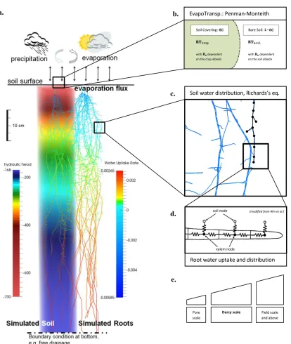
Figure 3: Schematic representation of the coupling of the Evapotranspiration, xylem transport and soil water modules. a) Soil pedon with the hydraulic head indicated in pseudo color (left) and three barley root systems (right) taking up water from that column. At the dry top water uptake is
negative, meaning that some hydraulic lift occurred in this scenario. b) The Penman-Monteith equation for simulating transpiration and evaporation. c) Zoomed version of roots, showing the edges and vertices. d) Network model for simulating water flow through the roots. e) Water transport in three dimensions in the soil is simulated by solving the Richards equation, which combines Darcy’s law with mass conservation, using the Finite Element Method.
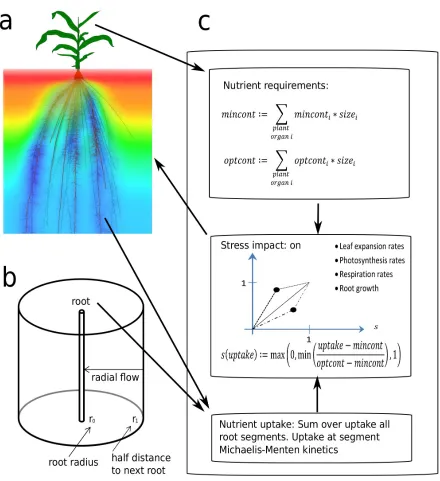
Figure 4: Schematic representation of the nutrient uptake, nutrient requirements and growth regulation modules. a) Root nutrient uptake coupled to model for solute transport in the soil. b) Schematic representation of the radial 1D Barber-Cushman model used for simulating P uptake. (c) summary of how the ratio between nutrient requirements and nutrient uptake determines plant physiology and/or growth.
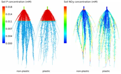
Figure 5: Simulation results for plastic and non-plastic root systems. Root plasticity was defined as increasing lateral branching density with increasing nutrient availability. Phosphorus availability (left two root systems) was high in the top soil, causing branching density to be high in the top as well. At the same time, the reduced branching density deeper down, due to plasticity, allows the plant to grow the individual laterals longer. Pseudo colors show the local phosphorus availability. Nitrate moves throughout the soil, and thereby the plasticity effect is less pronounced and difficult to trace (right two root systems).
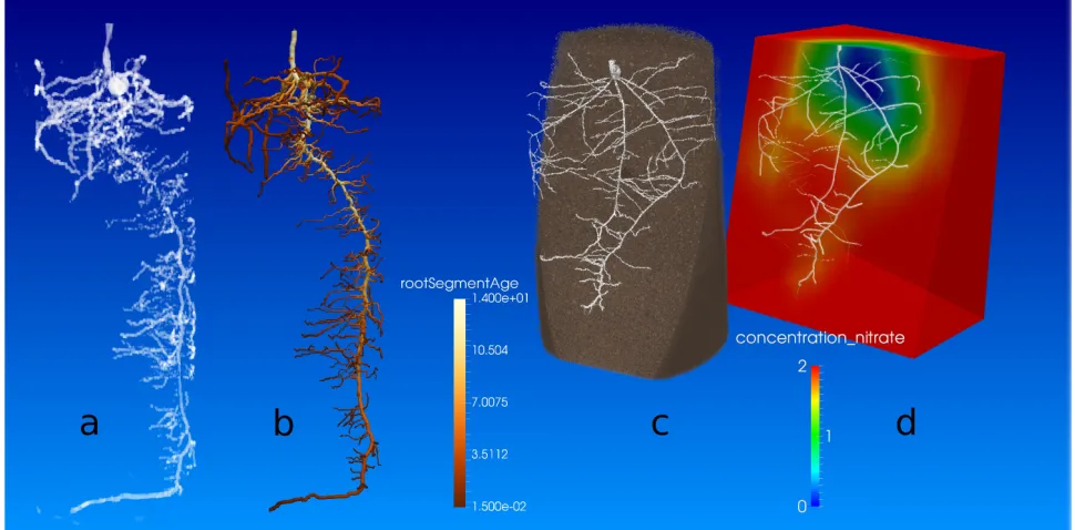
Figure 6: Simulation of imaged root phenotypes. a) Rendering of an MRI image of a two week old maize root system and b) the simulation of that root system by OpenSimRoot (right). Pseudo colors in 6b show the root segment age as estimated based on root topology, linear interpolation and the assumption that emergence of laterals takes two days. C) Rendering of segmented X-ray CT image 548
549 550 551
552 553 554 555
556 557 558 559 560 561 562 563
564 565 566 567 568
569 570 571 572 573 574 575
of a 10 day old wheat root system. Soil has been sliced to make roots visible. D) OpenSimRoot
simulation of the predicted nitrate depletion zone of in C imaged root phenotype. We assumed an initially homogeneous distribution of Nitrate within the simulated soil domain. Pseudo colors show the nitrate concentration on a plane cut approximately through the center of the root system.
Figure 1: Schematic representation of the OpenSimRoot code. Code encompasses three major components, the command line interface (CLI), different types of minimodels and a library of plugins. The class hierarchy for each component is given in Note S3.
Figure 2: Simulated root system of bean (left) and maize (right) as rendered with ParaView. Root systems are made up of different root classes, each with their own root diameter, branching rules, growth direction and growth rates. Root cross-sections are not simulated but illustrate root segment traits that are represented in OpenSimRoot.
584
585 586 587
588
[image:28.595.58.519.416.681.2]Figure 3: Schematic representation of the coupling of the Evapotranspiration, xylem transport and soil water modules. a) Soil pedon with the hydraulic head indicated in pseudo color (left) and three barley root systems (right) taking up water from that column. At the dry top water uptake is
negative, meaning that some hydraulic lift occurred in this scenario. b) The Penman-Monteith equation for simulating transpiration and evaporation. c) Zoomed version of roots, showing the edges and vertices. d) Network model for simulating water flow through the roots. e) Water transport in three dimensions in the soil is simulated by solving the Richards equation, which combines Darcy’s law with mass conservation, using the Finite Element Method.
593
594
Figure 4: Schematic representation of the nutrient uptake, nutrient requirements and growth regulation modules. a) Root nutrient uptake coupled to model for solute transport in the soil. b) Schematic representation of the radial 1D Barber-Cushman model used for simulating P uptake. (c) summary of how the ratio between nutrient requirements and nutrient uptake determines plant physiology and/or growth.
603
604
605 606 607 608 609
Figure 5: Simulation results for plastic and non-plastic root systems. Root plasticity was defined as increasing lateral branching density with increasing nutrient availability. Phosphorus availability (left two root systems) was high in the top soil, causing branching density to be high in the top as well. At the same time, the reduced branching density deeper down, due to plasticity, allows the plant to grow the individual laterals longer. Pseudo colors show the local phosphorus availability. Nitrate moves throughout the soil, and thereby the plasticity effect is less pronounced and difficult to trace (right two root systems).
611
Figure 6: Simulation of imaged root phenotypes. a) Rendering of an MRI image of a two week old maize root system and b) the simulation of that root system by OpenSimRoot (right). Pseudo colors in 6b show the root segment age as estimated based on root topology, linear interpolation and the assumption that emergence of laterals takes two days. C) Rendering of segmented X-ray CT image of a 10 day old wheat root system. Soil has been sliced to make roots visible. D) OpenSimRoot
simulation of the predicted nitrate depletion zone of in C imaged root phenotype. We assumed an initially homogeneous distribution of Nitrate within the simulated soil domain. Pseudo colors show the nitrate concentration on a plane cut approximately through the center of the root system.
619
620
New Phytologist Supporng Informaon
Arcle tle: OpenSimRoot: Widening the scope and applicaon of root architectural models
Authors: Postma, J.A.1, Kuppe, C.1 , Owen, M.R.2,3, Mellor, N.3,4, Gri'ths, M.3,4, Benne), M.J.3,4,
Lynch J.P.3,4,5, Wa), M. 1
1) Plant Sciences, Instute of Bio and Geosciences 2, Forschungszentrum Jülich, Wilhelm-Johnen Straße 52425 Jülich, Germany 2) Centre for Mathemacal Medicine and Biology, School of Mathemacal Sciences, University of No7ngham, UK
3) Centre for Plant Integrave Biology, University of No7ngham, UK
4) Plant & Crop Sciences Division, School of Biosciences, University of No7ngham, UK 5) Department of Plant Science, Pennsylvania State University, USA
Arcle acceptance date:
The following Supporng Informaon is available for this arcle:
Supplement 1 Descripon of the SimulaBase API
Supplement 2 How to run OpenSimRoot: descripon of CLI
Supplement 3 Example C++ code for a plugin
Supplement 4 Example C++ code for a plugin
Supplement 5 Technical descripon of water and nutrient modules
Supplement 6 Example input @le
Supplement 7 Example graph of state variables and their dependencies
Supplement 1: Application programming interface (API) of the SimulaBase
class
This interface is used by the plugins to navigate the hierarchy and retrieve necessary data. For an example see, Supplement 4. Developers that would like to develop a new plugin, will need this interface in order to retrieve data from other minimodels. These minimodels are in a hierarchy. The methods listed here can be used to find those minimodels in the hierarchy, and to request data from them. Minimodels are instantiations (objects) of class (type) SimulaBase.
//Method to retrieve meta data on a given minimodel such as its name, path in the hierarchy, lifetime of the object, and its units.
std::string getName()const; //name of object
std::string getPrettyName()const; //some what more humen readable name std::string getPath()const; //path to the object
virtual std::string getType()const; //What type this object has
bool evaluateTime(const Time &t)const; //check if t is within lifetime
Time getEndTime()const; //get the end time of object
Time getStartTime()const; //get the start time of object
virtual Unit getUnit(); //get the unit
void checkUnit(const Unit& unit)const; //check if unit equals given unit
void setUnit(const Unit &newUnit); //change unit
virtual void getXMLtag(Tag &tag); //get the object as tag (xml output)
//Methods to navigate the minimodel hierarchy
The difference between the get() and existing() methods is that when the object does not exist get() will throw an error and terminate the simulation, whereas existing() will return a NULL pointer. The getPath() methods will navigate a symbolic path just as a path in a filesystem is navigated. For example
getPath(“../mySib”) translates to getSibling(“mysib”), where the later is more efficient.
SimulaBase* getParent()const;
SimulaBase* getParent(const unsigned int i) const;
int getNumberOfChildren()const;//does not update!
int getNumberOfChildren(const Time &t);//does update
SimulaBase* getChild(const std::string & name,const Time & t);
SimulaBase* existingChild(const std::string & name,const Time & t);
SimulaBase* getChild(const std::string & name);
SimulaBase* existingChild(const std::string & name);
SimulaBase* getChild(const std::string & name,const Unit & u);
SimulaBase* existingChild(const std::string & name,const Unit & u);
SimulaBase* getSibling(const std::string & name,const Time & t);
SimulaBase* existingSibling(const std::string & name,const Time & t);
SimulaBase* getSibling(const std::string & name);
SimulaBase* existingSibling(const std::string & name);
SimulaBase* getSibling(const std::string & name,const Unit & u);
SimulaBase* existingSibling(const std::string & name,const Unit & u); //Sibling can be retrieved in alphabetic order.
SimulaBase* getNextSibling(const Time &t);