Robust stability analysis of LCL filter based synchronverter under different grid conditions

Robust Stability Analysis of LCL Filter Based

Synchronverter Under Different Grid Conditions

Roberto Rosso,

Student Member, IEEE

, Jair Cassoli, Giampaolo Buticchi,

Senior Member, IEEE

, Soenke

Engelken,

Member, IEEE

and Marco Liserre,

Fellow, IEEE

Abstract—Synchronverters have gained interest due to their

capability of emulating synchronous machines (SMs), offering self-synchronization to the grid. Despite the simplicity of the control structure, the adoption of an LCL-filter makes the overall model complex again, posing questions regarding the tuning of the synchronverter and its robustness. The inputs multi-outputs (MIMO) formulation of the problem requires multivari-able analysis. In this paper, the effects of control parameter and grid conditions on the stability of the system are investigated by means of structured singular values (SSV orµ-analysis). A step-by-step design procedure for the control is introduced based on a linearized small-signal model of the system. Then the design repercussions on the stability performance are evaluated through the performed robustness analysis. The developed linearized model is validated against time-domain simulations and labo-ratory experiments. These have been carried out using a power hardware-in-the-loop (PHIL) test bench, which allows to test the synchronverter under different grid conditions. As a conclusion the paper offers a simple guide to tune synchronverters but also a theoretical solid framework to assess the robustness of the adopted design.

Index Terms—Synchronverter robust stability analysis, µ

-analysis, synchronverter design, power hardware-in-the-loop tests.

I. INTRODUCTION

T

nected to the grid is growing noticeably causing con-cerns about the stability of the future power system. One of the main issues is related to the decrease of the total inertia of the system, but the risk of possible interactions between controllers of converters operating nearby cannot be underrated. Recent studies have shown that synchronization units of grid connected converters, usually phase-locked loops (PLLs), affect significantly the stability of the converters within their bandwidths [1]. Furthermore, interactions between synchronization units of power converters operating nearby have been observed and especially the fact that such effects are accentuated by weaker grid conditions [2]. During the last decade the concept of virtual synchronous machine (VSM) has been introduced [3]-[7]. Among the proposed control strategies, the synchronverter presented by Zhong et al. [5], [6] has been noted for its easy and intuitive structure and for

R. Rosso, J. Cassoli and S. Engelken are with Wobben

Re-search and Development (WRD) GmbH, Borsigstr. 26, 26607 Au-rich, Germany (e-mail [email protected], [email protected], [email protected]).

G. Buticchi is with the University of Nottingham Ningbo China (UNNC), 199 Taikang East Road, 315100 Ningbo, China (e-mail [email protected].)

M. Liserre is with the University of Kiel, Kaiserstr. 2, 24143 Kiel, Germany (e-mail [email protected]).

being the first proposed control algorithm in the literature for grid connected converters overcoming completely the need of a dedicated synchronization unit, both for initial synchronization to the main grid as well as during normal operation.

Synchronverter design has been recently addressed in sev-eral works [8]-[12]. Some of them rely on strong assumptions, such as grid short circuit ratio (SCR) higher then 10 in order to decouple active and reactive power loops [8]. Recent works presented tuning procedures based on reduced-order models of the system [10], [11]. Pole placement at prescribed locations in order to achieve desired dynamic has been proposed as optimal tuning procedure [11], [12] and eigenvalue analysis is the commonly adopted approach for investigation of stability of grid-connected converters and design purposes [13]. However, none of the works presented in the literature addresses robust stability analysis of the synchronverter. To this extent and according to the multi-inputs multi-outputs (MIMO) nature of the system, multivariable analysis is required [14], [15]. In fact, it is well known that eigenvalues are a poor measure of gain for MIMO systems, since they provide information about a specific system configuration and are not suitable for robust stability analysis and design of multivariable systems, where interactions between inputs and outputs of different channels take place [14].

It is common practice in the power electronics community to represent the grid as a Th´evenin equivalent with a restive-inductive impedance, whose parameters are calculated accord-ing to the short circuit power at the point of common couplaccord-ing

(PCC) and the estimated X/R ratio [16]. Unfortunately, this

representation might be often inaccurate since grid conditions change substantially during the day, due to the presence of other converters operating nearby or due to the variation of the number and characteristics of connected loads. An efficient way for modelling such effects would be to include uncer-tainties on the nominal plant. In this scenario, the structured

singular values (SSVs) analysis (commonly µ-analysis) has

been proven to be an efficient and reliable way for assessing robust stability of MIMO systems [14], [15], [17].

In this paper, the µ-analysis is performed to assess the

robust stability of an LCL grid connected synchronverter. The model developed in [10], based on linearized equations of the system, is adopted for the investigation. A design procedure of the synchronverter, using reduced-order models of active and reactive power loops is presented, which relys on nominal filter

parameters and grid conditions. Subsequently, the µ-analysis

𝑇𝑚+ −

𝑇𝑒

−

𝐷𝑝

1 𝐽𝑠

𝜔𝑟𝑒𝑓

ω 1

𝑠

Calculation

𝑣𝑖𝑟𝑡𝑢𝑎𝑙 𝑒𝑚𝑓

𝜃

PW

M

gen

er

at

io

n

1 𝐾𝑠

𝑄𝑠𝑒𝑡

𝐷𝑞

𝑒∗

𝑉𝑟𝑒𝑓

𝑀𝑓𝑖𝑓

− −

𝑄

+

-𝑅𝑓1 𝐿𝑓1

𝑅𝑐

𝐿𝑓2

𝐶

𝑅𝑓2 𝑅𝑔 𝐿𝑔

Filter

𝑖𝐿1 𝑖𝐿2

𝑖𝐶

𝑒 = 𝐸∠𝜃 𝑒𝑔= 𝐸𝑔∠ 0

1 𝜔𝑛

𝑃𝑠𝑒𝑡

1

𝜔𝑛 P and Q

Calculation

𝑣𝑃𝐶𝐶

𝑖𝑔 𝑃

Control

PCC Grid

+

-𝑣𝑐

Fig. 1. Simplified scheme of the system under study.

and grid conditions on the stability of the system. Through the performed investigation effects that are not clearly visible by means of an eigenvalue analysis are highlighted, especially the fact that synchronverters turn to be very robust against grid uncertainties under weaker grid conditions, which is exactly the opposite trend shown by grid connected converters using dedicated synchronization units [2].

The rest of the paper is structured as follows: in section II, the small-signal model of a synchronverter connected to the grid through an LCL filter along with the adopted control design procedure are introduced. Section III presents the concept of robust stability analysis by means of SSVs and its application to the system under study. In section IV, experimental results using a power hardware-in-the-loop (PHIL) test bench are shown, while section V is dedicated to the conclusions.

II. SMALL-SIGNALMODEL AND DESIGN

In the following, the small-signal model of a synchronverter connected to the grid through an output LCL filter presented in [10] is briefly introduced.

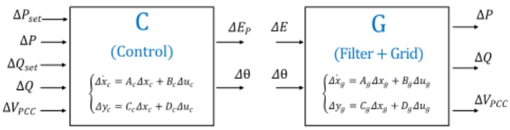
The model has been developed by splitting the overall system into two separated subsystems, namely the control and the plant composed of the filter and the grid. The simplified scheme of the system under study is depicted in Fig. 1, while in Fig. 2, inputs and outputs of the two linearized subsystems are shown. The design procedure presented in [10] is described in this section and is adopted in this work for tuning the parameters of the control.

A. Small-signal model

The synchronverter control structure shown in Fig. 1

con-tains separated loops for active powerPand a reactive power

C

(Control) Δ𝑃𝑠𝑒𝑡

Δ𝑄𝑠𝑒𝑡 Δ𝑃

Δ𝑄 Δ𝑉𝑃𝐶𝐶

𝛥𝐸

𝛥θ

Δ𝑃

Δ𝑄

Δ𝑉𝑃𝐶𝐶 𝛥θ

𝛥𝐸𝑃

𝛥𝑥 = 𝐴𝑐 𝑐𝛥𝑥𝑐+ 𝐵𝑐𝛥𝑢𝑐

𝛥𝑦𝑐= 𝐶𝑐𝛥𝑥𝑐+ 𝐷𝑐𝛥𝑢𝑐

𝛥𝑥 = 𝐴𝑔 𝑔𝛥𝑥𝑔+ 𝐵𝑔𝛥𝑢𝑔

𝛥𝑦𝑔= 𝐶𝑔𝛥𝑥𝑔+ 𝐷𝑔𝛥𝑢𝑔

G

(Filter + Grid)

Fig. 2. Inputs and outputs of the two linearized subsystems.

Q. The former emulates the frequency droop mechanism

typical of a SM described by the well-known swing equation:

Jω˙ =Tm−Te−Dpω , (1)

withJ representing the mechanical (virtual) inertia, ω the

virtual rotor speed, Dp the feedback gain accounting for the

(virtual) mechanical friction of the machine,Teis the electrical

torque and Tm is the mechanical one. Dp does not only

represent the virtual friction of the machine, but also the

active power-frequency droop coefficient of the controller.Tm

can be directly calculated from the active power setpointPset

simply by dividing by the nominal frequency ωn. The virtual

rotor angle θis obtained integrating ω and is needed for the

calculation of the virtual back-emf e∗. The reactive

power-voltage droop control reacts to a power-voltage deviation ∆V from

its nominal/reference value with a change of the reactive power

setpoint ∆Q, according to the droop coefficient Dq:

∆Q=−Dq∆V. (2)

The instantaneous reactive power measured at the output of the converter is then compared to its setpoint and added to the signal coming from the voltage droop. The resulting quantity

is processed through an integrator with gain 1/K producing

the virtual mutual fluxMfif, which multiplied by the virtual

rotor speedωproduces the amplitude of the virtual back-emf

Ep. Linearization of this product yields:

∆Ep=Mfif0∆ω+∆Mfif ω0, (3)

where quantities with subscript ”0” denote values at the operating point. The chosen state variables of the control

system are the virtual rotor rotational speedω, the rotor angle

θand the mutual flux Mfif.

The state-space representation of the plant composed of the

filter and the grid is obtained by choosing iL1, iL2 and vc of

Fig. 1 as state variables, namely filter current at converter side, filter current at grid side and capacitor voltage, respectively,

and writing the equations in dq coordinates. Linearization is



       

       

∆P=3₂(IL2d0∆vPCCd+VPCCd0∆iL2d+

+VPCCq0∆iL2q+IL2q0∆vPCCq)

∆Q=3₂(VPCCq0∆iL2d+IL2d0∆vPCCq+

−VPCCd0∆iL2q+IL2q0∆vPCCd)

∆VPCC=

VPCCd0∆vPCCd+VPCCq0∆vPCCq

q

V2

PCCd0+VPCCq2 0

, (4)

where∆vPCCd and∆vPCCq can be calculated as:



   

   

∆vPCCd=∆vcd+Rc(∆iL1d−∆iL2d)+

−Rf2∆iL2d−Lf2di_dtL2d +ω0Lf2∆iL2q ∆vPCCq=∆vcq+Rc(∆iL1q−∆iL2q)+

−Rf2∆iL2q−Lf2

diL2q

dt −ω0Lf2∆iL2d

, (5)

whereRf2andLf2represent the resistance and inductance

of the grid-side elements of the filter, respectively, whereasRc

is the capacitor damping resistance.

B. Control Design

The design procedure adopted in this work aims to the optimization of the step response characteristics of the system in terms of rise time, overshoot and settling time. Its intent is to provide a simple and intuitive approach for the design of the synchronverter when the characteristics of the filter and the grid are known, avoiding the designer to rely on a trial and error procedure. It considers active and reactive power loops separately and approximates the corresponding closed-loop transfer functions to simplified second-order equations. Control parameters are calculated setting a desired damping factor. In fact, it is known from control theory that the optimal dynamic response of a second-order system is obtained setting

the damping ratio to 1/√2 [19]. Therefore, control

parame-ters are simply calculated expressing the equivalent damping ratios of the reduced-order closed loop transfer functions in terms of plant and control parameters and chosen so as to obtain the desired damping ratio. Recently, another work on synchronverter design based on a reduced-order model has been presented in [11]. It is important to point out that the introduced simplifications may result in design errors, with repercussions on the performance of the system. In fact, as it will be shown in the following subsection, it is always rec-comended to check the dynamic performances of the system using a full-order model to be sure that they comply with the required specifications. Regarding stability assessment, since the two loops are considered separately and due to the MIMO nature of the system under study, even using the full-order transfer functions of the plant in the active and reactive power loops design might lead to erroneous results [14], [15], due to the fact that the cross-coupling effects between the two loops are neglected. For this reason, multivariable systems theory should be applied in order to properly design the control.

In the next section, the µ-analysis is performed in order to

assess the stability margin of the MIMO system under study against a defined set of plant uncertainties, once the control has been tuned according to the adopted design procedure. Subsequently, the effects of control parameters variations on

ΔT

𝐷𝑝

1 𝐽𝑠 −

(a)

Frequency droop loop

−

Δ𝝎 1 𝑠

Δθ

Filter + Grid

ΔP

Δ𝑃𝑠𝑒𝑡

Frequency droop loop

Δ𝝎

(b) 1

𝜔𝑛

ΔT

Fig. 3. (a) Simplified frequency droop loop, (b) simplified active power loop.

the stability of the system are estimated, such that the designer can find the most suitable compromise between dynamic performances and stability margin. In [10], three different cases with different grid and filter characteristics have been examined, in order to test the effectiveness of the proposed design procedure under different system conditions. In this paper, one of the cases examined in [10], whose parameters are reported in Table I, is taken as reference and used in the following to describe the adopted design procedure. In this work, the filter design is not explicitly addressed and filter parameters are obtained according to the filter design procedure presented in [18].

The parameters to be tuned are theP−f droop coefficients

Dp and the virtual inertia J for the active power loop along

with the Q−V droop coefficient Dq and the factor K of

the reactive power loop. Often droop coefficients are already fixed due to specifications on the steady-state response and

therefore onlyJandKcan be adjusted to improve the dynamic

behaviour. However, the adopted design procedure is valid even in case that the four parameters are freely adjustable.

In Fig. 3(a), the simplified scheme of the synchronverter frequency droop loop is shown, described by the following first-order transfer function:

∆ω

∆T(s) =

1

Dp

1+s _DJ

p

= Kf

1+sτf

. (6)

In Fig. 3(b), the simplified scheme of the active power closed-loop is reported. The plant composed of the filter and

the grid (indicated as G in Fig. 2) is described dynamically

by the transfer function ∆P

∆θ. Each of the input-output transfer

functions of G can be approximated by an equivalent

first-order transfer function by looking at the characteristics of the poles of the system, shown in Table II for simplicity. Two time constants identify the dynamic of the system, indicated

as τp1 andτp2in Table II. The transfer function ∆_∆P

θ of Gcan

be approximated to the following first-order transfer function:

PT1P(s) = Gp

1+sτre f p

, (7)

whereGPis the steady-state value of ∆_∆P

θ andτre f pthe time

constant of its dominant pole, namely τp1 for this case, as

can be determined by observing its step response. ChoosingJ

sufficiently small (e.g. τf ≈ τre f p/10), the frequency droop

Table I

PARAMETERS OF THE EXAMINED CASE

Description Symbol Value

Inverter rated power Sn(kVA) 300

Short circuit ratio SCR 20

Reactive-resistive ratio X/R 10

Line-to-line voltage VLL(Vrms) 400

Rated grid frequency fg (Hz) 50

Grid inductance Lg(pu) 0.05

Inverter-side filter inductor Lf1 (pu) 0.08

Grid-side filter inductor Lf2 (pu) 0.02

Grid resistance Rg(pu) 0.005

Inverter-side filter resistor Rf1(pu) 0.02

Grid-side filter resistor Rf2(pu) 0.02

Capacitor damping resistor Rc(pu) 0.18

Filter capacitor C(pu) 0.05

Table II

CHARACTERISTICS OF THE POLES OFG

Pole Damping Frequency

(rad/sec)

Time constant (sec)

(p1-p2) -94.8± j314 0.289 328 1.05e-2 (τp1)

(p3-p4) -842± j6930 0.120 6980 1.19e-3 (τp2)

(p5-p6) -842± j7560 0.111 7610 1.19e-3 (τp2)

Papp(s) =

1

T2

ps2+2ζpTps+1

, (8)

whereTpandζprepresent the inverse natural frequency and

the damping ratio, respectively:

Tp= s

τre f pωnDp

Gp

; ζp=

1 2

s

Dpωn

τre f pGp

. (9)

Assuming DP bounded in order to comply with

steady-state performance requirements, the damping of the simplified second-order active power loop transfer function cannot be

influenced otherwise [7]. In case that DPis freely adjustable,

it can be tuned so as to achieve ζP=1/

√

2.

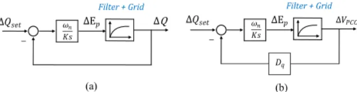
A Similar approach can be adopted for the tuning of the

reactive power loop. Due to the Q−V droop, two different

loops are identified, namely a reactive power and a voltage control loop, shown in Fig. 4(a) and (b) respectively.

−

ΔQ Δ𝑄𝑠𝑒𝑡 ΔE𝑝

(a) Filter + Grid

−

𝜔𝑛

𝐾𝑠

Δ𝑄𝑠𝑒𝑡 ΔE𝑝 Filter + Grid

Δ𝑉𝑃𝐶𝐶

𝐷𝑞

(b)

𝜔𝑛

𝐾𝑠

Fig. 4. (a) Simplified reactive power loop scheme, (b) simplifiedVPCCloop

scheme.

Also in this case, the behaviours of ∆Q

∆Ep and

∆VPCC

∆Ep of

G are approximated by reduced first-order transfer functions

indicated as PT1Q andPT1V, respectively:

PT1Q(s) = Gq

1+s τre f q

; PT1V(s) =

Gv

1+sτre f v

, (10)

where Gq and Gv are the steady-state values of

∆Q

∆Ep and

∆VPCC

∆Ep , respectively andτre f Q andτre f V are the time constants

of the respective dominant poles of each transfer function. The resulting damping factors of the two approximated transfer functions are reported below:

ζq=

1 2

s

K

τre f qωnGq

; ζv=

1 2

s

K

τre f vωnDqGv

. (11)

IfDqcan be arbitrarily modified, K andDq can be chosen

such that ζq=ζv=1/

√

2, otherwise the highest value of K

resulting from the two calculations is chosen.

Assuming that Dp and Dq are fixed to 5 % [20], the

calculated control parametersJopt andKopt for the case under

study are reported in Table III.

Table III CONTROL PARAMETERS

Parameter Value

Dp 60.8

Dq 18371

Jopt 6.38e-2

Kopt 37459

C. Simulation Results

Simulation results obtained using the full-order model of the system and setting the values of the control parameters accordingly to the adopted design procedure are shown in Fig. 5. Active and reactive power loops have been tested

separately and sweeps of Jand K are performed. Firstly, the

response of the system to a step ofPsetof 0.3 pu was observed

varying the value of J within the range

Jopt

50 ; 50 Jopt

,

whereas K was set to the calculated optimal value Kopt.

Subsequently, the response of the system to a step Qset of

the same amplitude was simulated varyingK within the range

Kopt

5 ; 5Kopt

, whereas J=Jopt.

The directions of the arrows indicate the increment of the corresponding parameters, the red curve is the response obtained by setting the parameters calculated using the adopted design procedure, whereas green curves are for values below the calculated optimal one and blue curves for values above it. In Fig. 5 (b), the steady-state value of the reactive power does not reach the given setpoint of 0.3 pu due to the voltage droop controller, which adjusts the reactive power according to the measured voltage at the PCC.

III. ROBUST STABILITY ANALYSIS

0 0.05 0.1 0.15 0.2 0.25 0.3 Time [s]

(a) 0

0.1 0.2 0.3 0.4 0.5 0.6

[pu]

Transfer Function ("_P/"_Pset)

0 0.05 0.1 0.15 0.2 Time [s]

(b) 0

0.05 0.1 0.15 0.2 0.25 0.3

[pu]

Transfer Function ("_Q/"_Qset)

J

K

Fig. 5. (a) Effects ofJon the dynamic behaviour of ∆P

∆Pset; (b) effects ofK

on the dynamic behaviour of ∆Q

∆Qset. (red): Response with the parameters from

design procedure, (green): response for values lower then the optimal one, (blue): response for values higher then the optimal one.

account the possible interactions between different channels that typically occur in a MIMO system. For accurate robust-ness assessment of MIMO systems, multivariable analysis is required and different methods have been developed, such

as the structured singular values (SSV) or µ-analysis [14],

[15], [17]. Singular values provide better information about the gains of the plants and the robustness of the control is verified against a defined set of system uncertainties. This method allows to span a set of possible system configuration instead of verifying stability only for a specific condition.

Parameter inaccuracies or non-linearities are among the most common sources of uncertainties. Other common sources of uncertainties are represented by neglected dynamics due to delays of sensors and/or actuators. These kind of uncertainty sources have a frequency dependent behaviour and can be included in the set of uncertain plants by using appropriate representations. The control loops of each grid connected con-verter modify the frequency behaviour of the equivalent grid seen by other converters operating nearby [13]. These effects can be also included in the stability analysis as uncertainties on the plant. The common way of modelling uncertainties is

to add perturbations to the nominal plant Gin an additive or

multiplicative way [14], [15]. The multiplicative representation consists on defining the set of perturbed plants as:

Gp=G(1+w∆); with k∆k∞≤1; (12)

where∆is a block diagonal normalized matrix including all

the possible perturbations, k∆k∞ represents its

H

wis a multiplicative weight. The multiplicative representation

is often preferred over the additive one, as the numerical values of its weights are more informative [14]. For example,

at frequencies where |w(jω)|>1, the uncertainty exceeds

100 %. Multiplicative uncertainties are characterized by a small amplitude for low frequency, increasing to unity and above at higher frequencies. This is a consequence of dynamic properties that inevitably occur in physical systems. Uncer-tainties might be located at the input or at the output of the plant. Input multiplicative uncertainty is suitable for modeling uncertain high frequency dynamics and uncertain right half plane zeros, while output inverse multiplicative uncertainty for low frequency parameter errors and uncertain right half plane poles [15]. In this work, the input multiplicative uncertainty representation is used in order to investigate the robustness

of the control against high-order frequency effects, such as resonant grid impedance behaviour or the effects of controllers of other power electronics converters operating nearby. A mul-tiplicative uncertainty weight is defined and, according to it, the robustness of the control is investigated varying controller parameters and grid conditions. The results are then compared to eigenvalue analysis, showing that the analysis performed with structured singular values enables highlighting effects that cannot be explicitly observed looking at the eigenvalues of the system.

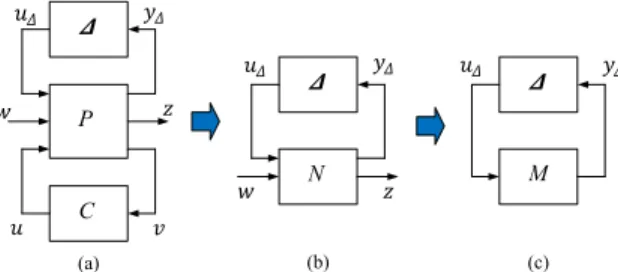
A. Problem formulation for µ-analysis

In order to perform the µ-analysis, the system should be

represented in the lower fractional transformation (LFT) form

[17]. This process is often referred to as ”pulling out the∆’s”

[15]. In Fig. 6 the steps required for bringing the system in a

form suitable forµ-analysis are shown. First, the uncertainties

have to be ”pulled out” from the plant and the system has to

be put in the form shown in Fig. 6 (a). Subsequently, theN∆

-structure shown in Fig. 6 (b) is obtained by means of a LFT

between the generalized plantPand the controllerC, defined

as [14]:

P

C

𝜟

N

𝜟 𝜟

M

𝑢 𝑣

𝑤 𝑧

𝑢𝛥 𝑦𝛥

𝑤 𝑧

𝑢𝛥 𝑦𝛥 𝑢𝛥 𝑦𝛥

(a) (b) (c)

Fig. 6. Problem formulation forµ-analysis: (a) general control formulation, (b) N∆-structure, (c) M∆-structure.

N=Fl(P,C)

∆

=P11+P12C(I−P22C)−1P21. (13)

Finally, theM∆-structure is simply derived considering that

M=N11. The structured singular value µ is defined as the

smallest structured∆(measured in terms of the largest singular

value σ (∆)), which makes the matrix I−M∆ singular; then

[14]:

µ(M)=∆ 1

min

∆

{σ |det(I−M∆) =0 f or structured ∆}. (14)

The inverse ofµ(M)can be interpreted as a stability margin

with respect to the structured uncertainty set affecting M.

This means that indicating the peak of µ(M) =β across the

frequency rangeω, stability is guaranteed for all perturbations

with appropriate structure and with respect to the chosen uncertainty, such that:

max

ω σ

(∆)≤ 1

β. (15)

B. Application to the system under study

A practical application ofµ-analysis to the studied system is

presented in the following. All the required calculations can be carried out by means of the ”Control System Toolbox”

of MATLAB [21]. The generalized plant P shown in Fig. 6

(a) can be obtained using the command sysic. The general

control formulation for the particular case under study is

shown in Fig. 7, where y∆=

z1 z2T, u∆=

w1 w2T and

the two multiplicative input uncertainties Wδ1 andWδ2 have

been located at the input channels u1 and u2. Outputs of P

are then the control inputs shown in Fig. 2 and represented

by the vectorv=

v1v2v3v4v5]. Using the starpcommand

from the same toolbox of MATLAB, the star product between

P andCcan be calculated, obtaining (13).

Δ𝑄𝑠𝑒𝑡 Δ𝑃𝑠𝑒𝑡

G

C Δ𝑃 Δ𝑄 Δ𝑉𝑃𝐶𝐶

Δ𝐸𝑝

Δ𝜗 P

W𝛿1

W𝛿2 𝛿1

𝛿2 𝑧1 𝑧2 𝑤1

𝑤2

𝑢1

𝑢2

𝑣1 𝑣3 𝑣2

𝑣4 𝑣5

𝑤3

𝑤4

Fig. 7. Construction of the generalized plant of the system under study.

101 102 103 104 105

Frequency(rad/s)

-10 -5 0 5 10 15

Magnitude(dB)

High-frequency uncertainty

Fig. 8. Multiplicative input uncertainty used for theµ-analysis.

In Fig. 8, the multiplicative input uncertainty used for the analysis is reported. It shows an amplitude of 50% at low frequency, increasing till 500% at very high frequencies. The chosen weight accounts for low frequency uncertainties due to parametric uncertainty in the model as well as high frequency neglected dynamic effects or resonant effects of the grid due to the presence of other converters operating nearby. Considering the system with the parameters listed in Table I and Table III,

in the following the effects of control parameters J andK as

well as gridSCRvariations on the eigenvalues of the systems

are shown and compared to the results obtained through the

µ-analysis.

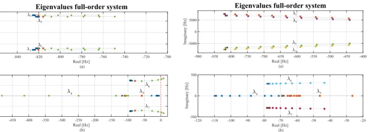
C. Variation of J

In Fig. 9 (a) and (b), the migration of the nine eigenvalues

of the full-order system due to a sweep of J in the range

Jopt

20 ; 20Jopt

is shown. The direction of the arrows indicate

Fig. 9. Effects of variation of control parameterJon the eigenvalues of the system, (a) migration ofλ1, (b) migration ofλ2-λ9.

100 ₁₀1 ₁₀2 ₁₀3 ₁₀4 ₁₀5

Frequency (rad/s)

0 0.2 0.4 0.6 0.8 1

Magnitude

7 factor - Mutliplicative INPUT uncertainty

J

J

Fig. 10. Behaviour ofµfactor due to variations ofJ.

the increase of the parameter J. Red points indicate the

loca-tions of the eigenvalues for reference condiloca-tions represented

byJ=Jopt,K=KoptandSCR=20, whereas green points are

for values ofJ<Jopt and blue ones for values ofJ>Jopt. It

is clear that the parameterJis mainly affecting the eigenvalue

λ1, causing a migration of the eigenvalue toward the imaginary

axis, whereas the other eight eigenvalues move leftwards.

In Fig. 10, the results of the µ-analysis are shown, where

colours have the same meaning as in Fig. 9. Under reference conditions, the control is quite robust against the defined

plant uncertainties. The maximum value of µ=0.6169 and

is reached at a frequency of 277 rad/sec. According to the

results shown in Fig. 10, an increase of J tends to augment

the robustness of the system at higher frequency, as can be also deduced from the eigenvalue analysis, since the dominant eigenvalues move leftwards. However, an excessive increase

of this parameter increases the peak of theµ factor at lower

frequencies, reaching almost the unity for J=20 Jopt. This

represents an important aspect that needs to be considered during the design procedure. In fact, it is common thought that VSMs should reproduce the inertia of a real synchronous machine of the same size. This requires the introduction of additional energy storage in the DC-Link of the converter, increasing sizes and costs. The results shown through this analysis indicate that generally high values of virtual inertia

J do not always correspond to an increment of the stability

Fig. 11. Effects of variation of control parameterJon the eigenvalues of the system, (a) migration ofλ2-λ5, (b) migration ofλ6-λ9.

100 101 102 103 104 105

Frequency (rad/s)

0 0.2 0.4 0.6 0.8 1

Magnitude

7 factor - Mutliplicative INPUT uncertainty

K K

Fig. 12. Behaviour ofµfactor due to variations ofK.

D. Variation of K

Fig. 11 (a) and (b) show the migration of the eigenvalues

due to variation of the parameter K. The parameter is varied

within the range

Kopt

5 ; 5 Kopt

. λ1 is far away from the

origin and is not relevantly affected. For values of K lower

thenKlim≈9000,λ6andλ7are located on the right half plane

causing instability.

The results of the µ-analysis shown in Fig. 12 indicate an

increase of the robustness of the system for higher values

of K at all frequencies. However, for values of K >Kopt

the stability margin is not relevantly enhanced. It is worth pointing out that, according to the chosen uncertainty weights,

the limit of µ=1 is reached for K≈19000, which is more

conservative if compared to the limit obtained through the eigenvalue analysis. This is simply explained by the fact that

µ provides information about robustness, covering a wide set

of possible plants, while eigenvalues show results only for one particular system.

E. Variation of grid SCR

Fig. 13 shows the migration of the eigenvalues due to

a decrease of the grid SCR from 20 to 2, when the X/R

ratio is set to 10. The direction of the arrows indicates the increase of the corresponding value, showing clearly that all the eigenvalues move rightwards when the impedance of the

Fig. 13. Effects of variation of gridSCRon the eigenvalues of the system, (a) migration ofλ2-λ5, (b) migration ofλ6-λ9.

100 101 102 103 104 105

Frequency (rad/s)

0 0.1 0.2 0.3 0.4 0.5 0.6 0.7

Magnitude

7 factor - Mutliplicative INPUT uncertainty

SCR

Fig. 14. Behaviour ofµfactor due to variations of the gridSCR.

grid is increased. This would lead to the consideration that the synchronverter is less stable when connected to a weaker grid. Similar conclusions have been drawn in [22], where the stability of a synchronverter-dominated microgrid has been investigated.

However, looking at the results of theµ-analysis reported in

Fig. 14, the decrease of the gridSCRhas instead the effect of

reducing theµfactor for all frequencies below≈1000rad/sec,

where the highest peak ofµis located. This indicates that the

control results to be more robust against the defined set of uncertainties shown in Fig. 8 when connected to a grid with higher impedance. This can be explained by the fact that the synchronverter behaves as a SM and basically as a voltage source behind an impedance. Indeed, stator inductances of SMs are usually much higher than typical converter filter inductances and their high impedance enhances the stability of the machine against high frequency perturbations [23].

It is worth to notice that the behaviour of the synchronverter highlighted through the performed analysis contrasts the trend of PLL-based converters, which instead result to be much more sensitive to perturbations in the plant (represented for example by the presence of other converters operating nearby) when connected to a weaker grid [2].

F. Considerations for synchronverter design

taken into account during the design procedure:

• In this work, control parameters have been tuned without

considering any requirements on virtual inertia. In fact, in the design procedure presented in the previous section,

J has been set to a proper low value so as to neglect

the dynamic of the frequency droop loop in the active power control loop. For the specific case under study, a

stability margin improvement is achieved for values ofJ

up to≈10Jopt. However, a further increase ofJ causes

a reduction of the stability margin of the converter at low frequencies.

• K affects significantly the stability of the converter. To

comply with the design procedure presented in the

pre-vious section, the highest value ofK resulting from (11)

has been selected asKopt. According to the results of the

performed stability analysis and observing the dynamic

behaviour shown in Fig. 5 (b), a further increase of K

over a certain limit simply worsen the dynamic perfor-mances of the converter, without significantly improving its stability.

• The performed analysis has pointed out that the stability

of the synchronverter against the defined set of high frequency uncertainties is augmented by the presence of high impedance between the converter and the grid. As already mentioned, stator inductances of SMs are much higher than usual converter filter inductances, typically designed so as to optimize the trade-off between power quality and size of the filter components [18]. A simple and efficient way for reproducing the characteristics of a SM by means of a VSC without necessarily increasing the size of the hardware components, is the emulation of virtual impedance through the control [23]. The use of virtual impedances is well-known in the literature and several techniques have been proposed for various pur-poses, e. g. harmonic suppressions [24], inverter currents limitation [25] or output admittance shaping [26], to name but a few. An overview on the techniques proposed in the literature is not the focus of this work, but rather highlighting that this expedient might be adopted in order to enhance the stability of the synchronverter [23]. Finally, one might think about including the stability anal-ysis shown in this paper as part of a comprehensive design procedure, which aims to find the best compromise between dynamic performances and stability margin. An example of a possible iterative process is reported in Fig. 15. The flowchart shown in Fig. 15 (a) summarizes the steps of the design method adopted in this paper and described in section II.B, whereas in Fig. 15 (b), the extended flowchart including stability margin considerations is depicted.

IV. EXPERIMENTALRESULTS

Laboratory experiments have been performed in order to validate the linearized model used for the analysis. In Fig. 16 (a), a simplified scheme of the experimental setup used for the tests is depicted, while in Fig. 16 (b), a picture of the labora-tory environment is shown. Each phase of a 4 kVA converter

Set Dp and Dq according to steady-state droop charcateristics (e.g. 5%)

Get nominal plant parameters (filter and grid) Design Process

Calculate J setting and K according to eq.(11)

𝜏𝑓≈ 𝜏𝑟𝑒𝑓1/10

Chech dynamic preformances of full-order model

End 𝑌𝑒𝑠

No

Chech dynamic preformances of full-order model

End

𝑌𝑒𝑠

No

Define plant uncertainty and check robust stability

𝑌𝑒𝑠 No

𝑌𝑒𝑠

No

(a)

(b) Design Process

Satisfactory dynamic performances?

Satisfactory stability margin?

Virtual impedance implemented?

Adjust value of K (higher K: slower response, more damping;

lower K: faster response, less damping)

Set Dp and Dq according to steady-state droop charcateristics (e.g. 5%)

Preliminary calculation of J setting and K according to eq.(11) 𝜏𝑓≈ 𝜏𝑟𝑒𝑓1/10

Modify plant parameters considering virtual impedance

Adjust value of J and/or K and eventually consider virtual

impedanceimplementation

Satisfactory dynamic performances?

Adjust value of K

(higher K: slower response, more damping; lower K: faster response, less damping)

Get nominal plant parameters (filter and grid)

Fig. 15. (a) Steps of design procedure adopted in this paper and proposed in [10], (b) extended design procedure including robust stability considerations.

Danfoss of the Series FC-302 is connected to a 4-quadrant linear power amplifier PAS 15000 from Spitzenberger-Spies (single phase rated power 15 kVA, total three phase rated power 45 kVA). The converter is additionally equipped with a transformer to provide galvanic isolation.

The principle of PHIL simulations is briefly explained in the following. A virtual grid is simulated by means of a real-time simulator (RTDS in the specific case). The simulator measures the converter currents at the PCC, corresponding to the currents flowing into the power amplifier. In the RTDS, a grid model runs in real-time, simulating the effects of the currents injected by the converter on the virtual grid. The simulated voltages at the PCC are sent to the power amplifier

to reproduce at its terminal the reference voltages provided by

the simulator almost instantaneously (slew rate>52 V/µsec).

This setup allows testing the behaviour of the converter under different grid conditions simply modifying the parameters of the grid model implemented in the simulator. The described setup has been used for validation of the model adopted for the analysis presented in this paper.

A resistive-inductive grid, as the one shown in Fig. 1, has been simulated in the RTDS and the parameters of the virtual grid have been modified so as to emulate a variation

of the grid SCR from 20 to 2 assuming a constant X/R ratio

of 10. The control has been tuned following the procedure described in this paper. Setup parameters are shown in Table IV. In Fig. 17, measurements results are compared to time-domain simulations in MATLAB/Simulink/PLECS (where a voltage source has been used to model the converter) and to analytical results obtained from the small-signal model. Steps of active and reactive power of 0.25 pu are shown for

three different values of SCR, namely 20, 10 and 2, whereas

the voltage control droop loop at the PCC has been either activated or deactivated. A good match between simulations and measurements can be appreciated. As already noticed in Fig. 5, the steady-state value of the output reactive power does not reach the given setpoint when the voltage droop is activated. This behaviour is much more accentuated for

lower SCR. The Q-V droop does not influence significantly

the dynamic of the active power steps and therefore in Fig. 17

only ∆P

∆Pset steps for the case when the voltage droop is activated

are shown.

Further experimental results are shown in Fig. 18, where

DC-Link Inverter LCL Filter Trafo PCC

Control

(a)

(b)

Power Amplifier

Grid Model 𝑉𝑃𝐶𝐶

𝐼𝑃𝐶𝐶

dSPACE

Power Amplifier

RTDS

Inverter

DC-Source

𝑇𝑚+

−

𝑇𝑒 −

𝐷𝑝

1 𝐽𝑠

𝜔𝑟𝑒𝑓

ω 1

𝑠𝜃

1 𝐾𝑠

𝑄𝑠𝑒𝑡

𝐷𝑞 _𝑉

𝑟𝑒𝑓 𝑀𝑓𝑖𝑓

− −

𝑄

1 𝜔𝑛

𝑃𝑠𝑒𝑡

1 𝜔𝑛 𝑃

𝑉𝑃𝐶𝐶

𝑉𝑃𝐶𝐶 𝐼𝑃𝐶𝐶

dSPACE RTDS

𝑅𝑔 𝐿𝑔

𝐸𝑔

𝐼𝑃𝐶𝐶 _𝑉 𝑃𝐶𝐶

𝑉 𝑃𝐶𝐶

𝑃𝑢𝑙𝑠𝑒𝑠

Fig. 16. (a) Scheme of the laboratory setup, (b) picture of the laboratory environment.

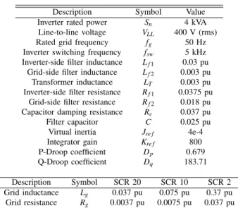
Table IV

PARAMETERS EXPERIMENTAL SETUP

Description Symbol Value

Inverter rated power Sn 4 kVA

Line-to-line voltage VLL 400 V (rms)

Rated grid frequency fg 50 Hz

Inverter switching frequency fsw 5 kHz

Inverter-side filter inductance Lf1 0.03 pu

Grid-side filter inductance Lf2 0.003 pu

Transformer inductance LT 0.003 pu

Inverter-side filter resistance Rf1 0.0375 pu

Grid-side filter resistance Rf2 0.018 pu

Capacitor damping resistance Rc 0.037 pu

Filter capacitor C 0.025 pu

Virtual inertia Jre f 4e-4

Integrator gain Kre f 800

P-Droop coefficient Dp 0.679

Q-Droop coefficient Dq 183.71

Description Symbol SCR 20 SCR 10 SCR 2

Grid inductance Lg 0.037 pu 0.075 pu 0.37 pu

Grid resistance Rg 0.0037 pu 0.0075 pu 0.037 pu

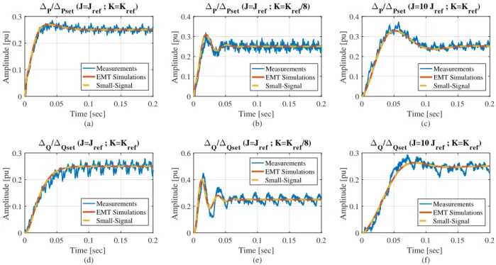
the parametersJ and K have been varied from the reference

values shown in Table IV. In Fig. 18 (b) and (e), the dynamic

responses of the system to steps of Pset and Qset of 0.25 pu

for K=Kre f/8 are respectively shown, whereas Fig. 18 (c)

and (f) show the response of the system forJ=10Jre f.

Looking at the results shown in Fig. 17 and Fig. 18, it can

be noticed how a decrease of theK value causes a reduction

of the high frequency damping of the system. An increase of

the virtual inertia factorJ tends to slow down the system in

terms of settling time and rise time. Additionally, an increase of the corresponding overshoot can be observed as well, indicating a reduction of low frequency damping. Operation of the converter has been tested even under extremely weak

grid conditions (SCR=2), which are typically critical for a

standard grid connected converter. It can be noticed how in this case the response of the system is simply slowed down,

but the light overshoot shown in the nominal case (SCR=20)

is eliminated instead. According to the presented results, one can conclude that the low frequency dynamic behaviour is not

worsened by the lowerSCR, which is instead the case for an

increase of the virtual inertiaJ.

V. CONCLUSION

In this paper, the robust stability analysis of a synchronverter connected to the grid through an output LCL filter is presented. A simple design procedure is introduced, which is used for tuning the control parameters according to nominal filter and grid characteristics. A robust stability analysis has been carried out based on the SSVs theory, which allows to assess the stability margin of the system according to a defined set of uncertainties. The effects of the variation of control parameters as well as grid characteristics on the stability of the

system have been observed. Through the preformedµ-analysis,

0 0.05 0.1 0.15 0.2 0.25 0.3 Time [sec]

(a) 0

0.1 0.2 0.3

Amplitude [pu]

"_P/"_Pset - SCR=20

Measurements EMT Simulations Small-Signal

0 0.05 0.1 0.15 0.2 0.25 0.3

Time [sec] (d) 0

0.1 0.2 0.3

Amplitude [pu]

"_Q/"_Qset - SCR=20 - Droop OFF

Measurements EMT Simulations Small-Signal

0 0.05 0.1 0.15 0.2 0.25 0.3

Time [sec] (b) 0

0.1 0.2 0.3

Amplitude [pu]

"_P/"_Pset - SCR=10

Measurements EMT Simulations Small-Signal

0 0.05 0.1 0.15 0.2 0.25 0.3

Time [sec] (e) 0

0.1 0.2 0.3

Amplitude [pu]

"_Q/"_Qset - SCR=10 - Droop OFF

Measurements EMT Simulations Small-Signal

0 0.05 0.1 0.15 0.2 0.25 0.3

Time [sec] (c) 0

0.1 0.2 0.3

Amplitude [pu]

"_P/"_Pset - SCR=2

Measurements EMT Simulations Small-Signal

0 0.05 0.1 0.15 0.2 0.25 0.3

Time [sec] (f) 0

0.1 0.2 0.3

Amplitude [pu]

"_Q/"_Qset - SCR=2 - Droop OFF

Measurements EMT Simulations Small-Signal

0 0.05 0.1 0.15 0.2 0.25 0.3

Time [sec] (g) 0

0.05 0.1 0.15

Amplitude [pu]

"_Q/"_Qset - SCR=20 - Droop ON

Measurements EMT Simulations Small-Signal

0 0.05 0.1 0.15 0.2 0.25 0.3

Time [sec] (h) 0

0.05 0.1 0.15

Amplitude [pu]

"_Q/"_Qset - SCR=10 - Droop ON Measurements EMT Simulations Small-Signal

0 0.05 0.1 0.15 0.2 0.25 0.3

Time [sec] (i) 0

0.05 0.1 0.15

Amplitude [pu]

"_Q/"_Qset - SCR=2 - Droop ON Measurements EMT Simulations Small-Signal

Fig. 17. Dynamic behaviour of ∆P

∆Pset, step of 0.25 pu: (a)SCR= 20, (b)SCR= 10, (c)SCR= 2. Dynamic behaviour of

∆Q

∆Qset, step of 0.25 pu, Q-V Droop

off: (d)SCR= 20, (e)SCR= 10, (f)SCR= 2. Dynamic behaviour of ∆Q

∆Qset, step of 0.25 pu, Q-V Droop on: (g)SCR= 20, (h)SCR= 10, (i)SCR= 2.

0 0.05 0.1 0.15 0.2

Time [sec] (a)

0 0.1 0.2 0.3

Amplitude [pu]

"

P/"Pset (J=Jref ; K=Kref)

Measurements EMT Simulations Small-Signal

0 0.05 0.1 0.15 0.2

Time [sec] (d)

0 0.1 0.2 0.3

Amplitude [pu]

"

Q/"Qset (J=Jref ; K=Kref)

Measurements EMT Simulations Small-Signal

0 0.05 0.1 0.15 0.2

Time [sec] (b)

0 0.1 0.2 0.3 0.4

Amplitude [pu]

"

P/"Pset (J=Jref ; K=Kref/8)

Measurements EMT Simulations Small-Signal

0 0.05 0.1 0.15 0.2

Time [sec] (e)

0 0.2 0.4 0.6

Amplitude [pu]

"

Q/"Qset (J=Jref ; K=Kref/8)

Measurements EMT Simulations Small-Signal

0 0.05 0.1 0.15 0.2

Time [sec] (c)

0 0.1 0.2 0.3 0.4

Amplitude [pu]

"

P/"Pset (J=10 Jref ; K=Kref)

Measurements EMT Simulations Small-Signal

0 0.05 0.1 0.15 0.2

Time [sec] (f)

0 0.1 0.2 0.3

Amplitude [pu]

"

Q/"Qset (J=10 Jref ; K=Kref)

Measurements EMT Simulations Small-Signal

Fig. 18. GridSCR= 20, Q-V droop off, X/R=10. Dynamic behaviour of ∆P

∆Pset, step of 0.25 pu: (a)J=Jre f,K=Kre f; (b)J=Jre f,K=Kre f/8; (c)J=10Jre f, K=Kre f. Dynamic behaviour of _∆∆_QQ_set, step of 0.25 pu: (d)J=Jre f,K=Kre f; (e)J=Jre f,K=Kre f/8; (f)J=10Jre f,K=Kre f.

against the trend shown by grid connected converters using a dedicated synchronization unit. The model used for the analysis has been validated against simulations and laboratory experiments using a PHIL setup.

REFERENCES

[2] R. Rosso, G. Buticchi, M. Liserre, Z. Zou, and S. Engelken, ”Stability analysis of synchronization of parallel power converters,” inProc. 43rd Annual Conference of the IEEE Industrial Electronics Society (IECON), Beijing, China, 2017, pp. 440-445.

[3] H.-P. Beck and R. Hesse, ”Virtual synchronous machine”, in Proc. 9th Int. Conf. on Electrical Power Quality and Utilization (EQPU), Barcelona, Spain, Oct. 2007, pp. 1-6.

[4] S. D’Arco, J. A. Suul, and O. B. Fosso, ”A virtual synchronous machine implementation for distributed control of power converters in smartgrids,”Int. J. Electric Power System Research, pp. 180-197, 2015. [5] Q.-C. Zhong and G. Weiss, ”Synchronverters: inverters that mimic synchronous generators,”IEEE Trans. Ind. Electron., vol. 58, no. 4, pp. 1259-1267, Apr. 2011.

[6] Q.-C. Zhong, P.-L. Nguyen, Z. Ma, and W. Sheng, ”Self-synchronized synchronverters: inverters without a dedicated synchronization unit,”

IEEE Trans. Power Electron., vol. 29, no. 2, pp. 617-630, Feb. 2014. [7] S. Dong and Y. C. Chen, ”Adjusting synchronverter dynamic response

speed via damping correction loop,”IEEE Trans. Energy Convers., vol. 32, no. 2, pp. 608-619, Jul. 2017.

[8] H. Wu, X. Ruan, D. Yang, X. Chen, W. Zhao, Z. Lv, and Q.-C. Zhong, ”Small-signal modeling and parameters design for virtual synchronous generators,”IEEE Trans. Ind. Electr., vol. 63, no. 7, pp. 4292-4303, Jul. 2016.

[9] M. Amin, A. Rygg, and M. Molinas, ”Self-synchronization of wind farms in an MMC-based HVDC system: a stability investigation”,IEEE Trans. Energy Conv., vol. 32, no. 2, pp. 458-470, Jun. 2017.

[10] R. Rosso, J. Cassoli, S. Engelken, G. Buticchi, and M. Liserre, ”Analysis and design of LCL filter based synchronverter,” inProc. IEEE Energy Conv. Congr. and Exp. (ECCE), Cincinnati, OH, 2017, pp. 5587-5594. [11] S. Dong and Y. C. Chen, ”A method to directly compute synchronverter parameters for desired dynamic response,”IEEE Trans. Energy Conv., vol. 33, no. 2, pp. 814–825, Jun. 2018.

[12] R. Aouini, B. Marinescu, K. B. Kilani, and M. Elleuch, “Synchronverter-based emulation and control of HVDC transmission,”IEEE Trans. Power Syst., vol. 31, no. 1, pp. 278–286, Jan. 2016.

[13] X. Wang, F. Blaabjerg, and W. Wu, ”Modeling and analysis of harmonic stability in an AC power-electronics-based power system,”IEEE Trans. Power Electron., vol. 29, no. 12, pp. 6421-6432, Dec. 2014.

[14] S. Skogestad and I. Postlethwaite, ”Multivariable feedback control -analysis and design”, Wiley and Sons, 2001.

[15] K. Zhou and J. C. Doyle,”Essentials of robust control”, Upper Saddle River: NJ. Prentice-Hall, 1998.

[16] L. Jessen, Z. Zou, B. Benkendorff, M. Liserre, and F. W. Fuchs, ”Resonance identification and damping in AC-grids by means of multi MW grid converters,” inProc. 42nd Annual Conference of the IEEE Industrial Electronics Society (IECON), Florence, 2016, pp. 3762-3768. [17] S. Sumsurooah, M. Odavic, and S. Bozhko, ”µ approach to robust stability domains in the space of parametric uncertainties for a power system with ideal CPL ,”IEEE Trans. Power Electron., vol. 33, no. 1, pp. 833–844, Jan. 2018.

[18] M. Liserre, F. Blaabjerg, and S. Hansen, ”Design and control of an LCL-filter-based three phase active rectifier”,IEEE Trans. Ind. Appl., vol. 41, no. 5, pp. 1281-1291, Sep. 2005.

[19] D. Schroeder,”Elektrische Antriebe 2, Regelung von Antriebssystemen”, 2nd ed., Germany: Springer-Verlag, 2001.

[20] P. Kundur, ”Power System stability and control”, McGraw-Hill, Inc. 1994.

[21] G. J. Balas, J. C. Doyle, K. Glover, A. Packard, and R. Smith”µ Analysis and synthesis toolbox”, Matlab user’s guide.

[22] Z. Shuai, Y. Hu, Y. Peng, C. Tu, and Z. J. Shen, ”Dynamic-stability analysis of synchronverter-dominated microgrid based on bifurcation theory,” IEEE Trans. Ind. Electr., vol. 64, no.9, pp. 7467-7477, Sep. 2017.

[23] V. Natarajan and G. Weiss, ”Synchronverters with better stability due to virtual inductors, virtual capacitors and anti wind-up,”IEEE Trans. Ind. Electron., vol. 64, no. 7, pp. 5994-6004, Jul. 2017.

[24] A. Terraso, J. I. Candela, J. Rocabert, and P. Rodriguez, ”Grid voltage harmonic damping method for SPC based power converters with multi-ple virtual admittance control,” inProc. IEEE Energy Conv. Congr. and Exp. (ECCE), Cincinnati, OH, 2017, pp. 64-68.

[25] X. Lu, J. Wang, J.M. Guerrero, and D. Zhao, ”Virtual impedance based fault current limiters for inverter dominated AC microgrids,” IEEE Trans. Smart Grid, vol. 9, no. 3, pp. 1599-1612, May 2018.

[26] X. Wang, Y. W. Li, F. Blaabjerg, and P. C. Loh, ”Virtual-impedance-based control for voltage-source and current-source converters,”IEEE Trans. Power Electron., vol. 30, no. 12, pp. 7019-7037, Dec. 2015.

Roberto Rosso (S’17) received his B.Sc. in

Elec-tronic Engineering and his M.Sc. in Electrical Engi-neering in 2009 and 2012, respectively from the Uni-versity of Catania, Italy. In 2013 he joined the R&D division of the wind turbine manufacture ENERCON (Wobben Research and Development WRD), where he is currently working in the control engineering department. He has been involved in several research projects addressing analytical models of electrical machines and control of electric drive systems. Since 2017 he is pursuing the Ph.D. in electrical engineer-ing at the Christian- Albrechts-University of Kiel, Germany. His research focuses on control strategies for grid integration of renewable energy systems.

Jair Cassoli received in 2006 his M.Sc. in

elec-trical engineering from the Technical University of Dresden, Saxony, Germany. He has been with ENERCON R&D division in Aurich, Germany, a wind energy converter manufacturer, since 2006 as development engineer. He is responsible for model based design power control strategies for wind en-ergy converters at the control system department. He has also been participating in collaboration with grid operators in several project specific studies concern-ing transient analysis of wind farm grid integration and protection based on EMTP modelling. His main research fields include control of electric machinery and drives for renewable energy systems and modelling and analysis of wind power plants connected to large power systems.

Giampaolo Buticchi(S’10-M’13-SM’17) received

the Masters degree in Electronic Engineering in 2009 and the Ph.D degree in Information Technolo-gies in 2013 from the University of Parma, Italy. In 2012 he was visiting researcher at The University of Nottingham, UK. Between 2014 and 2017 he was a post-doctoral researcher at the University of Kiel, Germany. He is now Associate Professor in Electrical Engineering at The University of Notting-ham Ningbo China. His research area is focused on power electronics for renewable energy systems, smart transformer fed micro-grids and dc grids for the More Electric Aircraft. He is author/co-author of more than 150 scientific papers.

Soenke Engelken(S’08-M’12) is the Head of

Con-trol Engineering at WRD Wobben Research and Development. The Control Engineering department develops control solutions for wind energy con-verters, spanning wind turbine controls, electrical systems controls and grid-side converter controls. Prior to joining Wobben Research and Development, he received his Ph.D. and M.Sc. degrees in control engineering from the University of Manchester, UK, in 2012 and 2008, respectively, as well as his B.Sc. degree in electrical engineering and computer sci-ence from Jacobs University Bremen, Germany, in 2007. He is a member of the IEEE Power and Energy Society, the IEEE Control Systems Society, of CIGR ´E Joint Working Group A1/C4.52 Wind Generators and Frequency-Active Power Control and of the ENTSO-E Expert Group on High Penetration Issues.

Marco Liserre (S’00-M’02-SM’07-F’13) received