Analysis Customer Support at 'payleven'

(1)

Analysis Customer Support

at ‘payleven’

Rob Kroezen

s0199494

[email protected]

Mechanical Engineering

(Production Management)

(2)

Management Summary

Due to the fast growth of the customer base of ‘payleven’, the number of inbound contact points is increasing. A further growth is expected; therefore the capacity of customer support (CS) should be sufficient to serve all merchants adequately. Management would like to get insight into the optimal staffing schedule for the current as well future situation while achieving the KPI’s that are set by global management. Therefore a simulation study that focuses on inbound calls is performed.

Research question

The main research question of this study is:

What is the optimal staffing schedule per day given a number of inbound calls per day that results in minimal personnel costs while the average queue time is below one minute and a minimum of 90% of the daily calls are answered.

The result of this study provides management of insight into optimal staffing schedules and therefore how to minimize personnel costs.

Result

By changing the agent-assigning rule the time agents are unoccupied are better distributed. By changing the allocation rule from ‘Random’ to ‘First predeces-sor’, the efficiency of the agents will increase.

By varying the incoming calls per day, optimal shift-configurations have been found. The optimal staffing schedules given a number of calls per day are: 175/225 calls per day:

• Two agents from 9:00 to 18:00 • One agent from 12:00 to 21:00 275 calls per day:

• Two agents from 9:00 to 18:00 • One agent from 9:00 to 12:00 • One agent from 12:00 to 21:00 325 calls per day:

• Three agents from 9:00 to 18:00 • One agent from 12:00 to 21:00 375 calls per day:

• Three agents from 9:00 to 18:00 • One agent from 9:00 to 12:00 • One agent from 12:00 to 21:00

The results also give an insight into the trade-off between working hours and the targets. Based on the figures, management can make a discussion whether to increase the working hours to achieve a better service level.

(3)

Introduction

This report is the result of my internship ‘Operations’ at ‘payleven’. The main goal of the internship was to optimize the back-office activities at the Benelux office of ‘payleven’. The daily activities involved were:

• Manage and improve the complete RMA-process for PIN-readers that re-turn under warranty

• Offering second tier support to the department ‘Customer support’ • Provide detailed transactional specifications for merchants

• Extensive mobile app-testing for new releases

In the last months of the internship, the main focus was shifted towards pro-viding management of a detailed insight in optimal staffing schedules for the department ‘Customer support’. Therefore a simulation study that focuses on inbound calls is performed. This report is all about the simulation study done during my internship.

Acknowledgments

(4)

About ‘payleven’

The company ‘payleven’ [6] provides a mobile Chip & Pin-solution. It offers a flexible and secure solution with transparent costs for small and medium-sized businesses. It is a great alternative for existing PIN-solutions that mostly come along with a yearly contract and fixed costs.

[image:4.595.200.401.263.465.2]

The Chip & PIN card reader, that is shown in figure 0.1, connects to a smart-phone or tablet via Bluetooth and is managed through the payleven app.

Figure 0.1: The Chip & PIN card reader and a smartphone with the payleven-app

(5)

1 Introduction of the problem

Merchants of ‘payleven’ [6] can contact customer support in several ways. For instance they can send an email, chat on Livechat [3] or, like most merchants do, make a phone call.

Due to the fast growth of the customer base of ‘payleven’, the number of inbound contact points is increasing. A further growth is expected; therefore the capacity of customer support (CS) should be sufficient to serve all merchants adequately. Management would like to get insight into the optimal staffing schedule for the current as well future situation while achieving the KPI’s that are set by global management. Therefore a simulation study that focuses on inbound calls is performed.

The main research question of this study is:

What is the optimal staffing schedule per day given a number of inbound calls per day that results in minimal personnel costs while the average queue time is below one minute and a minimum of 90% of the daily calls are answered.

The result of this study should help management to get insight into optimal staffing schedules and therefore minimize personnel costs.

1.1 Approach

First the current situation is modeled and analyzed. The model is verified and validated by for instance statistical tests. Then several experiments are designed and performed. The types of shifts and the number of incoming calls are varied.

The results of the designed experiments are used to determine the performance indicators per setup, so the average queue time, the number of working hours and the percentage of calls that is answered. From this data an optimal config-uration given a number of incoming calls is determined. The results are then extensively discussed.

1.2 Expected result

The simulation-study will give insight into:

• An optimal staff schedule given a number of calls per day • The number of working hours for each studied configuration • Average queue time per studied configuration

(8)

2 Model description

In this section information on the model is given. An explanation will be given on what tasks the focus lies on and which things are restricted and cannot be changed. Then a brief explanation on the simulation model and its verification and validation is given. At the end of this chapter it will be clear which as-sumptions are done and how the model is constructed to answer on the research question.

2.1 Scope

The tasks of CS are summarized below;

• Inbound calls, when a (potential) customer has got a question, he can contact ‘payleven’ by phone. This is the most common way that customer support is contacted.

• Livechat [3], during opening- hours a chat-window is available on the web-site of ‘payleven’ [6].

• Email, in case of a question, a customer can send an email that should be answered within 24 hours.

• Outbound tasks, on a daily basis customer support calls customers for several reasons, for instance when a customer did not use the pin-reader for a while (reactivation call) or if a transaction failed (transaction-failure call).

The main focus of this study is on the inbounds tasks of CS due to the non-deterministic characteristics of it. The outbound tasks that for instance needs te be done, are set by global management and are therefore better predictable. So these tasks are not included in the model. Furthermore, the inbound calls provides the bulk of the work. The email tasks are not included because they take significantly less time than the inbound tasks. In practice the Livechat tasks are combined with other tasks for an employee. The output of the model will be generated such that the head of CS will be able to estimate if an employee has got enough capacity left to deal with other tasks; for each modelled agent the time he is unoccupied is recorded.

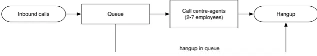
[image:8.595.137.454.599.655.2]

In figure 2.1 a schematic overview of the system that is modelled, is given.

Figure 2.1: General overview system

(9)

inbound calls. When there are no agents available, the calls are stored in a First Come First Serve way. When an agent becomes available, the call is immediately transferred to the agent. In case there are multiple agents available the call is randomly assigned to an agent. After a call has been completed, a note in the CRM-software (Customer relationship management) Salesforce [7], should be made. There are 30 seconds available to do this, after it, the agent is automatically put on available again.

2.2 Level of detail

The following parameters are taken into account:

• The arrival rate of calls, an estimation is done on how the calls are dis-tributed per hour, this is elaborated in appendix B

• Percentage of customers leaving the system before their call is answered (hangup in queue), this is explained in section 3.2.2

• The distribution of the time per call, several probability distributions have been hypothesized and tested, eventually empirical data is used in the model, this is explained in appendix C

• Average time a call stays in the queue, this is a result of the number of agents that are available, the abandon rate and the time per call

• The number of shifts per day, these are actually varied and the perfor-mance is measured

• The time that agents are (un)occupied, when there is a large portion of the shift-time that an agent is unoccupied, it means he can possibly be planned for additional activities (e.g. Livechat or mail)

The model is limited to certain restrictions;

• Opening times are 9:00 to 21:00 during the week and 10:00 to 18:00 on Saturday, however the main focus is on the weekdays due to the higher workload. The weekends are left out of the study

• There are standard shifts with fixed begin en end times, the shifts are not longer than 9 hours

• A 9-hour shift includes a break of 45 minutes • In the evening, minimal 1 agent should be planned

2.2.1 Assumptions

Some assumptions have been done to simplify the model, these are described below.

(10)

• Retry calls, are calls where a customer that hangs up, calls back later. These are not taking into account separately but are seen as independent calls.

• No redirections are modeled, so one call is always served by one agent. • The waiting capacity in the buffer is unrestricted.

• The calls arrive according a Poisson-process where the time between events is exponentially distributed withλ. More information on how the average number of calls per hour are determined, can be found in appendix B The prediction of the number of calls per week and day is beyond the scope of this study. However, an estimation of the distribution of the workload per day is made and explained in appendix B.

• The wrap-up time is the time after a call that is necessary to conclude a case. The standard time that is set in the real system is 30 seconds but this might vary because an operator can put himself on available earlier on. However, it is assumed that on average the wrap-up time is 30 seconds and thus is implemented as a fixed 30 seconds

• Staff illness and equipment failure are not taken into account, it is expected these events will only occur very rarely and will therefore have only minor impact. During the start of the day it frequently happens an operator cannot login due to for instance a forgotten password, but the head of CS will make sure these issues are prevented.

• A simplified method for determining the calls that abandon the system is made, this is explained in section 3.2.2.

• The weekends are left out of the study as described earlier on.

• The calls that will be left in the system after 21:00 pm are neglected. It is expected that this will not make a significant difference because the number of calls between 20:00 and 21:00 is low.

2.3 Experimental factors

The experimental factors that have been used, are explained here. These are categorized as either a resource or process intervention.

2.3.1 Resource interventions

The experimental factors that relate to resources are mainly based on staff-resources. The factors that will be varied are:

(11)

[image:11.595.186.408.175.253.2]

• The types of shifts per day, several types of shifts are available, by finding the optimal combination, the targets will be met while minimizing the working hours

Figure 2.2: Overview of current standard shifts

2.3.2 Process interventions

The main focus is on changing the number of available resources per day. How-ever, there is one process intervention studied, namely the way of distributing calls to the agents. Currently the calls are assigned randomly to agents. It is expected that, by changing this rule to, the occupation levels can be enhanced.

2.4 Performance indicators

The goal of the simulation is to find the optimal staffing schedule while the requirements are met. So the performance indicators are;

• Total working hours per day • Average waiting time in queue • % of calls answered

Furthermore, the utilization per agent per day is calculated. This is done to determine how much time an agent got left to do other CS-tasks. With this data head of CS can optimally plan the total number of agents for all the tasks that should be done.

2.5 Programming

The call-center is translated into a simulation model in Tecnomatix Plant Sim-ulation [8]. A description of the technical model can be found in Appendix A.

2.6 Verification

(12)

is checked and verified according the expectations. Furthermore, a visual check is performed by observing the animation.

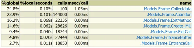
[image:12.595.133.462.265.347.2]

The ‘profiler’ in Plant Simulation is used to analyze the run time per method. For instance it became clear that that one method contributed for more than 90 percent to the total runtime. The implementation of this method was improved. After the improvement, the runtimes per method are explainable. In table 2.3 it can be seen the most time intensive method is ‘Collectdata’, this method is executed at the end of every replication, which means at the end of every day. It summarizes all data in the tables and writes them them to a table where the data per replication is recorded.

Figure 2.3: Final results of profiler for verification purposes

The most advanced method is the ‘abandon’ method. It is executed every minute and loops over the calls in the buffer and statistically determines if the callers hangs up. The method is verficated by changed the abandon-rate, for instance by setting the percentage to 0 % no calls should leave the system, this is indeed the case.

To check the use of common random numbers, two runs of the same configu-ration are compared. From the table 2.4 it can be seen that two runs give the same results.

[image:12.595.195.398.493.639.2]

(13)

2.7 Validation

By doing statistical tests to check assumptions it is checked that if model is a good representation of reality. Furthermore, empirical data has been used. The time per call is modelled by using empirical data that is defined as a fre-quency table. On first hand, a probability distribution was assumed, but after making graphical plots and performing a goodness of fit test, it is concluded no suitable probability distribution is found and empirical data is used. The explanation on this process is given in Appendix C.

As described in the chapter 2.2.1 a poisson-process for the arrival rate is as-sumed. The argumentation is given in appendix B. Empirical data is used to generate the arrivals.

(14)

3 Experimental design: factors & range,

assump-tions

This chapter describes which experiments are performed. Furthermore it will be clarified in which way the shifts of the agents are varied.

3.1 Type and settings of simulation

Before going on with the motivation for the experiments, a brief explanation on the settings and terminology is given:

Server - a server is defined as a processor in the plant simulation model, the processor represents one agent to which one shift is assigned.

Configuration - a new configuration is a setup where there is at least one differ-ence in shift type for one of the servers. The current shift types were given in section 2.3.1.

Simulation type - The simulation is of the type ‘terminating’ because each day the same initial condition (empty system) and same terminating event (closing time) occurs. The model is build up such that the system is empty after 21:00. The calls that will be left in the system after 21:00 pm are neglected. It is expected that this will not make a significant difference because the number of calls between 20:00 and 21:00 is low.

Number of replications - In the model a replication equals one day since CS closes every night. One simulation run in the model consists of multiple replica-tions. A statistical analysis is done to determine the number of replicareplica-tions. All experiments will consist of 100 replications. The calculations and a motivation for this number of replications can be found in appendix D.

Simulation run - So one simulation run consists of 100 replications. The number of runs equals the number of configurations that are simulated.

3.2 Factors, range & assumptions

The experimental factors that are varied are the number and types of shifts per day. First the current situation is described and it is explained in which range the experimental factors are varied. As the number of incoming calls changes, other configurations are studied. In this section is described how these are determined.

3.2.1 Agent assigning rule

(15)

[image:15.595.176.406.186.378.2]

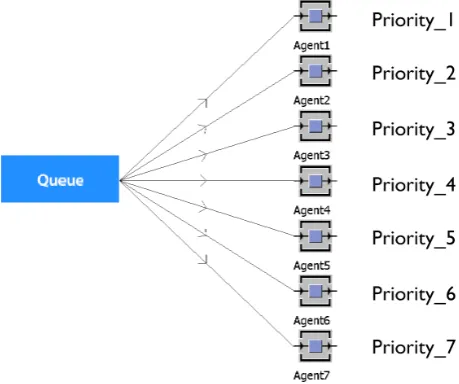
predecessor’. In the last method, a call is assigned with priority to an agent. It is always checked if a call can be moved to agent1, then to agent2 and so on. A schematic overview of the priority rule is given in figure 3.1.

Figure 3.1: A schematic overview of the priority rule

Before the other experiments are performed, it is concluded which setting gives the best results.

3.2.2 Abandon rate

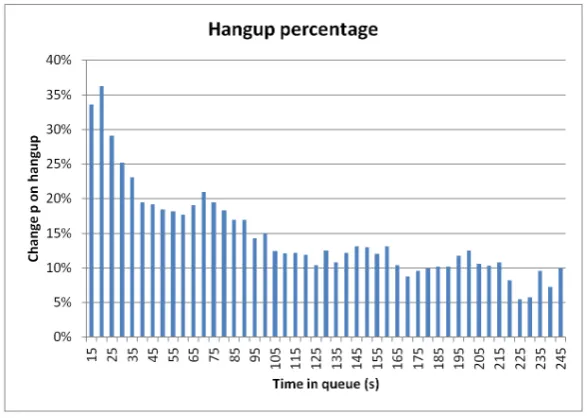
Based on empirical data, an estimation for the abandon rate is done. First the data-set is split into answered and unanswered calls. Then the chance that a customer hangs up the phone, based on the queue time, is calculated. This is plotted and can be seen in figure 3.2. The used data can be found in the Excel-sheet ‘Hangup frequency’.

The results have been discussed with head of CS according who the high hangup frequency for low queue times can be explained by outbound calls. A large percentage of outbound calls are not answered, however, because CS call with a call ID, the merchant can see who has been calling. A lot of customers call back, but when they hear the automatic voice-recorder within the first 5 seconds they hangup.

(16)

[image:16.595.150.444.125.334.2]

Figure 3.2: Percentage of customers that hangup given a queue time

3.2.3 Current situation - 225 calls per day

Currently the number of incoming calls is approximately 225 per day. To reduce the number of configuration to study, following assumptions are done;

• The shift from 9:00 to 18:00 is always occupied by a minimum of 2 agents, with less agents there is far too low capacity to meet the targets

• Between 9:00 and 18:00 a maximum of 3 agents have to be present for inbound tasks, when scheduling more agents there is overcapacity • In the whole day a maximum of 4 agents are necessary, when scheduling

more agents there is overcapacity

These assumptions are verified based on the output results. Under these as-sumptions no clear under- of overcapacity occurs, so the asas-sumptions are valid.

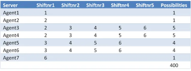
The possible shift numbers, that correspond to the shifts in figure 2.2, are given in table 3.3.

(17)

[image:17.595.141.454.128.243.2]

Figure 3.3: Overview of possible shifts per agent

Configuration 1 • Agent 1 - shift 1 • Agent 2 - shift 2 • Agent 3 - shift 3 • Agent 4 - shift 4

Configuration 2 • Agent 1 - shift 1 • Agent 2 - shift 2 • Agent 3 - shift 4 • Agent 4 - shift 3

3.2.4 Other situations - 175 calls per day

In case of a fallback of the average number of calls per day, less capacity is necessary. A situation where there are on average 175 calls per day, is studied. The same assumptions as described in the previous section 3.2.3 are applied. This is done because else under-capacity is expected. Therefore the variations as described in table 3.3 are also used for this scenario.

3.2.5 Other situations ->275 calls per day

(18)

[image:18.595.142.454.202.318.2]

Figure 3.4: Overview of possible shifts per agent when>275 calls

[image:18.595.139.454.498.615.2]

(19)

4 Analysis of results

4.1 Agent assigning-rule

The two settings for the distribution of the calls to the agents that are studied, are ‘Random’ and ‘To first predecessor’. When the last method is applied, it is always checked if a call can be moved to agent1, then to agent2 and so on. Both setups are simulated. To compare both methods, there are 3 configurations selected that meet the targets, the detailed results can be found in the Excel-file ‘CallCenterPayleven results’. In table 4.1 an overview is given.

Figure 4.1: Overview of selected expirements to determine best assigning-rule

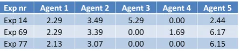
[image:19.595.173.422.538.590.2]

The tables 4.2 and 4.3 give the results for both settings. In table 4.2 the times that the agents are not calling are about the same. For instance when you look at experiment 14, agent 1 and 2 are respectively 4.1 and 4.2 hours unoccupied. The breaks of 0.75 hours should be deducted from both figures, however, this still leaves a large portion of time the agent is not calling.

[image:19.595.175.420.632.685.2]

Table 4.3 shows that when the calls are first moved to the first predecessor, the time that the agents are not calling, are more uneven distributed while the total time the agents are unoccupied remain approximately the same. When you compare for instance experiment 69 the results for both methods show a significant difference in the time agent 5 is unoccupied. In the current situation he has got 4.79 hours left for other activities, while in the case this is 6.17 hours. It should be noted that agent 1 has got left less time in the adapted case, but this gives an intended positive effect; it means agent 5 will be less disturbed and can thus do other tasks (e.g. chat/mail) more efficiently. Also agent 1 will be more occupied, which also increases his efficiency.

Figure 4.2: Time per agent (hours) not occupied (Method: Random)

(20)

So it is concluded the method ‘To first predecessor’ results in better performance. Therefore it is advisable the settings in NVM are adapted such. In all the following experiments, calls are assigned to agents based on the method ‘first predecessor’.

4.2 Selecting optimal configuration

The most optimal configuration is each time selected from the output that is gen-erated by the experiment manager (as explained in appendix A. The results of all the experiments can be found in the Excel-file ‘CallCenterPayleven results’. This sheet gives additional information for instance on the expected overtime per agent. Bases on these figures, extra tasks can be assigned to a shift (e.g. Livechat or mail).

By following the steps as below, the most optimal configuration is each time selected:

1. Sort results based on total working hours

2. Exclude all results where average waiting time in the queue>60 seconds 3. Exclude all results where the % answered calls is<90%

4. Find experiments with lowest working hours

5. Select the experiment with the highest % of calls answered

The next best configuration can be found by excluding the optimal configuration and the duplicates (some runs have done multiple times as described in section 3.2.3). Then repeat the steps as indicated above.

By following these steps, the most optimal configuration according the main research question, is found.

4.3 Current situation

In the next section the results are discussed.

4.3.1 225 calls

The best configurations when there are 225 calls are given in table 4.4. The corresponding shifts are given in table 4.5. Unfortunately experiment 16 is a non-feasible solution because it contradicts the restriction that in the evening minimal one agent should be present. This leaves experiment 32 as best run, and experiment 36 as second best.

The most optimal staff schedule when there is an average of 225 calls expected, is

(21)

[image:21.595.150.443.125.187.2]

Figure 4.4: Overview of best configurations (225 calls)

Figure 4.5: Overview of performance of best configurations (225 calls)

The expected % of calls that are answered is 90.91%. The expected average waiting time is 51.12 seconds.

By adding an extra shift from 9:00 to 12:00 the percentage of calls that is answered increases to 95.75% and the average queue time decreases to 24.98 seconds. A trade-off can be made between service level and costs.

4.3.2 175 calls

[image:21.595.125.468.581.631.2]

The best configurations when there are 175 calls are given in table 4.6. Unfor-tunately experiment 48 violates the restriction of having minimal one agent in the evening. Therefore, the best configuration is as in experiment 70.

The most optimal staff schedule when there is an average of 175 calls expected, is:

(22)

4.4 New situations

When the customer base of ‘payleven’ grows, additional phone calls can be expected. The estimation of the increase of phone calls is beyond the scope of this study. Therefore, the optimal configurations are determined for 275, 325 and 375 calls. These configurations are simulated and the results are explained in this section.

4.4.1 275 calls

[image:22.595.150.444.361.418.2]

The best configurations when there are 275 calls are given in table 4.8. The optimal configuration is experiment 128. Experiment 78 is not a sufficient solu-tion because there is no agent in the evening present. By adding an extra shift from 9:00 to 12:00 a pickup rate of almost 94% is achieved.

• Two agents from 9:00 to 18:00 • One agent from 9:00 to 12:00 • One agent from 12:00 to 21:00

4.4.2 325 calls

(23)

[image:23.595.152.443.125.185.2]

because there is no agent in the evening present. Therefore experiment 182 is the best alternative.

• Three agents from 9:00 to 18:00 • One agent from 12:00 to 21:00

4.4.3 375 calls

The best configurations when there are 375 calls are given in table 4.12. The best configuration is experiment 24. Experiment 14 is not a sufficient solution because there is no agent in the evening present. Therefore experiment 34 is the best alternative.

(24)

(25)

5 Conclusion

A simulation study that focuses on inbound calls is performed. The main research question of this study is:

What is the optimal staffing schedule per day given a number of inbound calls per day that results in minimal personnel costs while the average queue time is below one minute and a minimum 90% of the daily calls are answered.

By running several experiments the optimal staffing schedules for the current as well future situations are determined.

5.1 Results

The study has shown that by changing the agent-assigning rule the time agents are unoccupied are better distributed. By changing the allocation rule from ‘Random’ to ‘First predecessor’, the efficiency of the agents will increase. By varying the incoming calls per day, optimal shift-configurations have been found. The optimal staffing schedules given a number of calls per day are: 175/225 calls per day:

• Two agents from 9:00 to 18:00 • One agent from 12:00 to 21:00 275 calls per day:

• Two agents from 9:00 to 18:00 • One agent from 9:00 to 12:00 • One agent from 12:00 to 21:00 325 calls per day:

• Three agents from 9:00 to 18:00 • One agent from 12:00 to 21:00 375 calls per day:

The results can be used to make the most optimal staffing schedule. The detailed results indicates the time an agent is unoccupied. This can be used to assign other tasks (e.g. Livechat or mail) to the planned agents.

(26)

5.2 Recommendations

Mainly there are two recommendations, the first recommendation is changing the allocation-rule in NVM to ‘First predecessor’. This will increase the effi-ciency of the agents. The second recommendation is to plan the agents according the results as indicated above. This results in minimal personnel costs. By mak-ing use of the detailed results as given in the Excel-files, it can be estimated how many extra tasks an agents can complete.

5.3 Future research

It might be possible to find better configurations by changing the begin- and end times of the shifts. In this study, the shifts-times are assumed fixed, but by adding other standard shifts, better results may be found.

By performing a study on the number of incoming calls, that depends for in-stance on seasonal effects, a model that predicts the expected number of calls can be made. By doing this, it will be easier to determine the best staffing schedule.

(27)

(28)

A

Model description

Below an explanation on the model that is programmed in ‘Siemens Plant Sim-ulation’ [8], a discrete-event simulation tool, is given. A complete overview of the model can be found in appendix E.

A.1 Customer support

In figure A.1 can be seen how the actual call center is modeled. The system con-sists of a processor ‘Incomingcalls’. The calls are created, according the arrival distribution, on this processor by the method ‘CreateMU’ which is elaborated in appendix A.3. Then the call arrives in the queue. If an agent is available, the call is forwarded immediately. When there are no agents available, the call remains in the buffer in a First Come First Serve way. The calls are handled on the single processors ‘Agent1’, ‘Agent2’ and so on. After the call is completed, it is moved to the drain ‘HangUp’.

[image:28.595.148.443.398.599.2]

On each move of a call, one of the methods in the bottom of figure A.1 is triggered. When one of these methods is triggered, it assigns the current time to the call. When the call leaves the system, the times are stored into a table by the method ‘ExitMethod’.

Figure A.1: Customer support

A.2 Event control

(29)

[image:29.595.209.382.205.348.2]

A day-generator starts every day at 9:00; it initiates a day and runs the method ‘Startday’. Several daily-parameters are reset, for instance the counter of the number of customers in the system. Furthermore it cleans the daily tables. An ‘ExperimentManager’ is used to run the different configurations. To make sure the right shifts are set for the agents, an ‘Init’-method is added.

Figure A.2: Event control

A.3 Control & settings

The control & settings part contains the method that generates a ‘Moving unit’ (call) on the source-processor. The method is triggered by the MU-generator that is repeatedly activated with an interval that is set by the parameterλ. The

λvalue is changed hourly according the table ‘LambdaArrivals’. The reasoning on the choice ofλcan be find in appendix B.

The part contains a table with the data of the histogram as described in ap-pendix C.6. These values are used by the ‘servers’.

Also the abandoning-method is present, it is triggered every 1-minute interval by the ‘Abandon-generator’. For every call in the queue, the method stochastically determines if it will remain in the system or abandons it.

[image:29.595.154.438.565.634.2]

(30)

A.4 Shiftparameters

[image:30.595.230.365.232.446.2]

This section of the model contains all the shift-parameters. There are modelled as ‘ShiftCalenders’ that are assigned to a server based on the variables that are also present in the same part. The variables are set by the experiment-manager so several configurations can be simulated one after another automatically. It also contains a table where the working hours per shift are set, this is used to calculate the total working hours per configuration.

Figure A.4: Shifts parameters

A.5 Performance output

(31)

[image:31.595.211.381.326.497.2]

(32)

B

Arrival rate distribution

[image:32.595.140.453.227.392.2]

The number of calls vary week to week, this can be seen in figure B.1 that show the number of calls for a part of 2014. It is correlated to the season, but also to new product updates or other situations. The prediction of the number of calls per week is beyond the scope of this study. However, an estimation of the distribution of the workload per day should be made.

Figure B.1: Number of calls per week

It is assumed that the calls arrive according a Poisson-process where the time between events is exponentially distributed withλ. This seems a valid assump-tion because the arrival times are most likely independent. Furthermore, the implicit assumption is made that the distribution of the workload per hour is equal of all days.

The parameter λ stays constant for an hour and is then updated according a table. To determine aλfor each hour of the day given a total number of calls per day, historical data of 5 weeks is used (week 46-50). In the selected period (week 46-50) no unusual events occurred.

The average number of calls per hour is calculated. From this, the percentage of the total calls per hour is calculated. It can be seen that the most calls arrive between 11:00 and 12:00.

(33)

[image:33.595.144.449.332.495.2]

(34)

C

Distribution of time per call

Historical data is used to find a probability distribution for the time per call. Data of 5 weeks is used; the total of data points cq. number of calls is 5221. It is assumed the size of the set is sufficient and an adequate representation of the actual call-times. In the selected period (week 43-47) no unusual events occurred that may have led to shorter or extra long call-times. Below are the steps described to determine a distribution.

C.1 Hypothesizing of function

[image:34.595.151.445.344.542.2]

To decide what kind of distribution appears to be appropriate to fit the data, the data is divided in to bins and plotted as a histogram, the result can be seen in figure C.1. Also a statistical summary of the data can be found below in figure C.2. The positive skewness indicates that the data can be fitted with a Gamma, lognormal or Weibull-function [1].

Figure C.1: A histogram of the time per call

C.2 Parameter estimation

First, a Gamma-function is analyzed. The parameters of the distribution are estimated according;

α= µ

2

σ2 =

301.74717492

274.3067112 = 1.210078541 (C.1)

β= σ

2

µ =

274.3067112

(35)

[image:35.595.229.363.137.316.2]

Figure C.2: Statistical summary of the data

[image:35.595.149.444.421.608.2]

The historical data of the times per call is sorted. For each data point a chance P is calculated. A plot of the times per call as a function of P, together with a plot of the assumed gamma-distribution is made and is shown in figure C.3. The plot indicates that the Gamma-distribution might be a good fit.

Figure C.3: The sorted data plotted against a hypothesized Gamma-function

C.3 Q-Q plot

(36)

[image:36.595.150.442.149.332.2]

performed.

Figure C.4: Q-Q plot of empirical data versus hypothesized gamma-function

C.4 Chi-square test

The computations of the test can be found in the excel-sheet ‘Distribution-TimesPerCall’, the result is χ2_{= 387}_._{87. Looking up the chi-square value with}

α= 0.05 andυ= 72 gives aχ2

(72;0,95)= 92.80.

Because the chi-square of the empirical data is higher than the theoretical value the difference is statistically different so the assumption of a gamma-distribution is rejected.

C.5 Identification other individual distributions

To identify other potential distributions that can be used to fit the data, a study in Minitab 17 [4] is performed. The empirical data is imported in Minitab. Then through Stat - Quality tools - Identification individual distributions, several other distributions are evaluated based on their p-value.

If the p-value is lower than 0.05 it is concluded that the data does not follow the specified distribution. In figure C.5 the results can be found. It seems no appropriate fit can be found.

C.6 Empirical distribution

(37)

[image:37.595.192.397.136.276.2]

Figure C.5: Overview hypothesis testing other distributions

As can be seen in the excel-sheet ‘DistributionTimesPerCall’ the tail of the histogram is quite long. This is due to some calls with very long calltimes. These outliers have been discussed with the head of CS. Most of the time it seems these outliers are due to inexperienced CS-employees who were not able to help the customer adequately. Therefore extreme values (>2000 s.) are removed from the data and a new histogram is determined. The result can be seen in the figure C.6. The histogram is used as a frequency table in Plant Simulation.

[image:37.595.151.443.429.600.2]

(38)

D

Number of replications (sequential method)

To determine the minimum number of replications per run, where a replication is one day, a statistical analysis is performed. This appendix explains how the analysis is performed and what number of replications is used.

As described in section 3.1 the simulation is of the type ‘terminating’. Because one of the main performance indicators is the average waiting time in the queue, the sequential method is applied on this indicator.

The question is: how many replications are required such that an acceptable relative error is achieved. The relative error is: γ =|X−µ|/X. Aγ equal to 0.1 is a common figure.

When usingγ for our estimate of the relative error, the actual relative error is at mostγ/(1−γ). Therefore a corrected value is used γ0 =γ/(1−γ).

Starting from a number of replications of 2 each time the confidence interval as below is calculated. The goal is to find the number of replications for which the width of the interval is sufficiently small. The width of the confidence interval is equal to:

δ(n, a) =tn−1,1−α/2

p

S2

n/n (D.1)

A common value forαis 0.05 [1] and is used to find the t-values. The standard deviation Sn is calculated from the output data. As long as δ(n, a) > γ0, an extra replication is necessary. When δ(n, a) is equal to or smaller than γ0 a sufficient number of replications are performed. The calculations can be found in the excel-file ‘SequentialMethod’.

(39)

(40)

References

[1] Ph.D. Averill M. Law. Simulation Modeling and Analysis. McGraw-Hill, 2015.

[2] Rocket Internet. Website rocket internet. https://www.rocket-internet.com, 04 2015.

[3] Livechat. Website livechat. http://www.livechatinc.com, 04 2015. [4] Minitab. Website minitab 17. http://www.minitab.com, 04 2015.

[5] NVM. Website new voice media. http://www.newvoicemedia.com, 04 2015. [6] payleven. Website payleven. www.payleven.nl, 04 2015.

[7] Salesforce. Website salesforce. https://www.salesforce.com, 04 2015.

Analysis Customer Support at 'payleven'