Abstract—This comparative study focuses on various transformation methods of diversifying natural data to coded data. The findings provide the usefulness of obscuring confidential data and the widespread implementation of expedient methods of expanding product and process improvement. The natural data are generated via computer simulation under specific conditions of Taguchi experimental designs in forms of orthogonal arrays with and without noise. There are five transformed methods which include Box-Cox, Arcsine, Logit, Dual-power and Parabolic. Performance measures of the transformation methods are carried out via the ratio of signal-to-noise and an analysis of mean. Both of them are used to compare data analyses of all transformation methods for three cases of smaller-the -better, larger-the-better and target-the-better. Taguchi orthogonal arrays with and without noise are also considered results to compare influence of each capability of transformation methods. Furthermore, there is a determination of feasible ranges of transformation parameters to accomplish more suitable outcomes from natural data.
Index Terms—Taguchi Orthogonal Array, Signal-to-Noise, Analysis of Mean, Transformation Method.
I. INTRODUCTION
AGUCHI experimental design and analysis are a combination of statistical methods developed by Taguchi and Konishi [1]. Taguchi method has been widely utilised in engineering analysis. It is a planned experiment with the objective of acquiring data in a controlled way, in order to obtain information about the behavior of a given process. The greatest advantage of this method is the saving of effort in conducting experiments; saving experimental time, reducing the cost and discovering influential factors quickly. The effects of many different factors on the performance characteristic in a condensed set of experiments can be examined by using the orthogonal array experimental design proposed by Taguchi [2]. Furthermore, this method involves identification of proper controllable factors to obtain the optimal results of the process or product improvement. Orthogonal Arrays (OA) are also used to conduct a set of experiments. Results of these experiments are used to analyse the data and predict the quality of components produced [3]. Recently, this method has also Manuscript received December 11, 2014; revised January 10, 2015. The authors wish to thank the Faculty of Engineering, Thammasat University, THAILAND for the financial support.
*Nattapat IMSAP is with the Industrial Statistics and Operational Research Unit (ISO-RU), Department of Industrial Engineering, Faculty of Engineering Thammasat University, 12120, THAILAND, [Phone: 662-564-3002-9; Fax: 662-564-3017; e-mail: [email protected]].
Pongchanun LUANGPAIBOON is an Associate Professor, ISO-RU, Department of Industrial Engineering, Faculty of Engineering Thammasat University, 12120, THAILAND [[email protected]].
been immensely employed in several industrial fields and research works.
Diagnosing to transformed data, it was advantage for many businesses, commerce and manufacturing processes to obscure secretive data. They can not only indicate information to public but also the confidential data are prevented in terms of coded data. Data transformation applies a mathematical modification to covert a variety of possible data such as adding constant
,
raising or squaring to a power, and converting to logarithm scales etc. There are several researches related to the data transformation techniques since Box and Cox [4] presented the classical one of analysis of transformations via the lambda (λ) selection method for a power transformation. Osborne [5] used Box-Cox transformation to improve the efficacy of normalising and variance equalising for both positively- and negatively-skewed variables. Duran [6] has studied the use of Arcsine transformation in the analysis of variance (ANOVA) when the data follow a binomial distribution. The Monte Carlo simulation technique was used to generate the natural data. The results suggested that the transformed analyses do not always performed in better type I error. In some cases they lose the power and this provided some evidences to discourage the routine application of the Arcsine transformation in ANOVA. Rephael and Andrian [7] used Box-cox transformation in problem of Bayesian model and variable selection for linear regression which are considered transformations of response and predictor. He proposed that quantities, referred to as generalized regression coefficients, have a similar interpretation to the usual regression coefficients on the original scale of the data. Furthermore, variable and transformation selection were also uncertainty involved in the identification of outliers in regression. Thus, he used a more robust model to account for such outliers based on a t-distribution with unknown degrees of freedom. Parameter estimation is carried out using an efficient Markov chain Monte Carlo algorithm.This research compares five transformed methods which consist of Box-Cox, Arcsine, Logit, Dual-power, and Parabolic transformations. All methods are performed in cross Taguchi orthogonal arrays with and without noise factors in order to study how transformed methods with optimal values of transformed variables of
λ
for Box-Cox,Ω
for Arcsine and Logit, δ for Dual-power, and β for Parabolic affect the analytical result. Moreover, the influence of uncontrollable factors with and without noise factors are measured in Taguchi method against capability of each transformation is also determined.A Comparative Study of Analysing Transformed
and Noisy Data in Taguchi Orthogonal Arrays
Nattapat Imsap
*and Pongchanun Luangpaiboon,
Member, IAENG
II. TAGUCHI METHOD
A. General Review
Taguchi method is normally used to cover two related ideas. The first is that, by the use of statistical methods concerned with the analysis of variance. The experiments may be constructed which enable an identification of the important design factors responsible for degrading the product performance. The second (related) concept is that when judging the effectiveness of designs, the degree of degradation or loss is a function of the deviation of any design parameter from its target or nominal value.
Taguchi design is a set of methodologies by which the inherent variability of materials and manufacturing processes has been taken into account at the design stage. The application of this technique had become widespread in many US and European industries after the 1980s. The beauty of the Taguchi design is that multiple factors can be considered at once. Moreover, it seeks nominal design points that are insensitive to variations in production and user environments to improve the yield in manufacturing and the reliability in the performance of a product. Therefore, not only controlled factors can be considered, but noise factors as well. Although similar to the design of experiment (DOE), the Taguchi design only conducts the balanced (orthogonal) experimental combinations, which makes the Taguchi design even more effective than a fractional factorial design [8].
The philosophy of Taguchi is broadly applicable. He proposed that engineering optimisation of a process or product should be carried out in a three-step approach (Fig. 1), i.e., system design, parameter design, and tolerance design [9].
Fig. 1. Taguchi design procedures.
B. Signal-to-noise
Taguchi loss function or the quality loss function maintains that there is an increasing loss on both for producers and for the society at large. It is a function of the deviation or variability from the ideal or target value of any design parameter. The greater the deviation from target, the greater is the loss. The concept of loss being dependent on variation is well established in the design theory. At any
systems influential process levels are related to the benefits and costs associated with dependability when the output or response or the target value are analysed in the loss function. This quality loss function is given by the expression: l(yi)k(yi )2 (1) where
l(yi) is the loss function of output at value yi.
i
y is the measured quality of value
is the target value k is the constant
Expected values of the loss function consist of two statistical variables which are the sample variance (S2)and the squared of deviation from the mean of the target value via n samples. This concept leads to create performance measures of Taguchi method or the signal-to-noise ratio (S/N), which consist of three cases:
(i) smaller-the-better; the ideal target value is defined as zero.
n
1 i
2 i y n 1 log 10 S N /
S (2)
(ii) larger-the-better; it is preferred to maximise the result and the ideal target value is infinity.
n
1 i yi2
1 n 1 log 10 L N /
S (3)
(iii) target-the-better; there is a defined target value for the product or process which has to be achieved. There are specified upper and lower limits with the target specification being the middle point. Quality measure is, in this case, defined in terms of a deviation from the target value.
2 S
2 y log 10 T N /
S (4)
Furthermore, in this case there are two specified variables which are upper and lower limits. It has to designate just one variable affecting to the mean or the target value. Consequently, an additional measure via an analysis of mean (ANOM) can provides a confidence interval of the approach to compute upper and lower decision lines. In this case, we need to use analysis of mean to decide the adjustment variables for approaching to the target whereas the S/N drives the process or product characteristics.
C. Taguchi orthogonal array
An orthogonal array (more specifically a fixed element orthogonal array), denoted by OAN (sm), is an N×m matrix whose columns have the property that in every pair of columns each of the possible ordered pairs of elements appears the same number of times. The symbols used for the elements of an orthogonal array are arbitrary. The symbols of s, m and N are the number of factor levels, the number of factors and the number of test runs, respectively [10]. This paper uses two types of orthogonal array in Taguchi experimental design to create natural data which are L4
orthogonal array of 23 or OA4(23)for uncontrollable factors (m, n, o) with (-1, 1) of (low, high) levels (outer array or System design Determine suitable working levels of the design factors
Select proper Orthogonal array (OA)
Run experiments
Analyse data
Identify optimal condition
Confirmation runs
Determine the results of parameter design by tightening tolerance of
significant factors Tolerance design
noise) as shown in Table I, and L9 orthogonal array of 34 or
[image:3.595.330.549.43.208.2]OA9(34) for controllable factors (A, B, C, D) with (-1, 0, 1) of (low, medium, high) levels of the inner array as shown in Table II.
TABLE I
L4 ORTHOGONAL ARRAY OF 23 (OA4(23))
TABLE II
L9 ORTHOGONAL ARRAY OF 34 (OA9(34))
III. DATA TRANSFORMATION
Data transformations are commonly-used tools that can serve many functions in quantitative analysis of natural data (N), including improving normality of a distribution and equalising variance to meet assumptions and improve effect sizes, thus constituting important aspects of data cleaning and preparing for your statistical analyses. There are as many potential types of data transformations as there are mathematical functions. Some of the more commonly-discussed traditional transformations include: adding constants, square root, converting to logarithmic (e.g., base 10, natural log) scales, inverting and reflecting, and applying trigonometric transformations such as sine wave transformations [11-12].
Box and Cox transformation method or BC [4] is shown below:
0 ; y ln y
0 ; 1 y
1 y T y
(5)
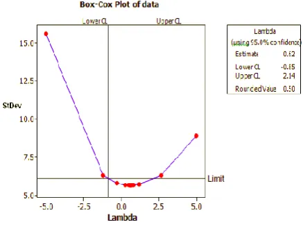
whereyny is a geometric mean of observations, n is total number of observations. This method selects the optimal level of λ (Fig. 2) which refers to lowest pooled standard deviation of Sp is given by an expression below:
i
) 1 i n ( i j
2 i y ij y p
S
(6)
Fig. 2. Relationship of pooled standard deviation and λ via Minitab program
Arcsine transformation method or AS [6] or the inverse sine of a square root of the proportion (p) is shown below:
) p ( e arcsin T
y (7) .
Logit transformation method or LG is defined as the logarithm of the odds. If p is the probability of an event, then (1–p) is the probability of not observing that event and the odds of the event are p/(1–p). The Logit transformation is most frequently used in logistic regression and for fitting linear models to categorical data. Thus, Logit method is
p 1
p log ) p ( it log T
y (8)
According to Arcsine and Logit methods are required proportion (p), this research defines the proportion (p) of
y/Ω, where y is the simulated data and Ω is the transformed variable.
Dual-power transformation method or DP [13] is shown below:
0 ; y log
0 ; y y T y
(9)
where:yTis the transformed data by the dual power transformation and δ is the power of the transformation methods.
Parabolic transformation method or PB is shown below: yT (y)2 (10)
where: yT is the transformed data by parabolic transformation and β is adding constant of the transformation methods.
IV. EXPERIMENTAL PROCEDURES
The natural data (y) are generated from linear statistical model with two case of L9 orthogonal array 34 and L9×L4
orthogonal cross array 34×23as shown in the equation and
Table below.Moreover, the level of standard deviation (σ) and mean of natural data (), which are used in this model are 1.0 and 25, respectively.
Experimental Number
Uncontrollable Factors (Outer Arrays)
m n o
1 -1 -1 -1
2 -1 +1 +1
3 +1 -1 +1
4 +1 +1 -1
Experimental Number
Controllable Factors (Inner Arrays)
A B C D
1 -1 -1 -1 -1
2 -1 0 0 0
3 -1 +1 +1 +1
4 0 -1 0 +1
5 0 0 +1 -1
6 0 +1 -1 0
7 +1 -1 +1 0
8 +1 0 -1 +1
[image:3.595.69.266.106.412.2]A case of OA without noise factors; ij e D 5 . 1 C 2 B 5 . 0 A 5 . 3
y (11)
A case of OA with noise factors;
3.5A 0.5B 2C 1.5D y ij e Bn o 5 . 1 n 5 . 0 m
[image:4.595.53.286.53.504.2]2 (12)
TABLE III
L9 ORTHOGONAL ARRAY
TABLE IV
L9xL4 ORTHOGONAL ARRAY
In the computational experimental design of Taguchi, there are two steps for finding data results. At the beginning, the defined data in all conditions were simulated by Minitab program while Matlab program were encoded in the same conditions. Then, results after running both programs were compared the signal-to-noise ratio (S/N) and the analysis of mean (ANOM) in two cases of performance measures of Taguchi method. It aims to assure the encoded program was valid. Finally, coding in Matlab was run repetitiously for finding the optimal transformed variable levels. The predefined feasible ranges of
λ
for BC and δ for DP are -5 to 5. The feasible ranges ofΩ
for AS and LG are 0 to 500, and
feasible ranges of parameter (β) for PB are -1000 to 1000. There are 100 replicates in experimental results for measuring distribution data of different analysis of mean and signal-to-noise results.V. EXPERIMENTAL RESULT AND ANALYSIS
The experimental results in case of Taguchi orthogonal array with and without noise factors were generated by running codes from Matlab program. They are collected as shown in Table VI, and Table VII. In case of OA with noise factors, ithas signal-to-noise (smaller-the-better,
larger-the-better, target-the-better) and analysis of mean results Conversely, the case of OA without noise factors has only analysis of mean result. In Taguchi orthogonal array without noise, it is shown that all transformation methods have not the ranking result similar to natural data. Box-Cox and Dual-power have the results much closer to natural data than the rest and only these two methods have optimal transformed variables.
TABLE V
ANOM RESULT OF OA WITHOUT NOISE FACTORS
[image:4.595.322.556.179.333.2]In this case, the transformed variables are furthermore calculated and measured the optimal levels in BC and DP. Another three methods have not optimal transformed variables from experimental results but range of transformed variable, which return the same result of analysis of mean, are also determined. The optimal transformed variables of BC and DP are calculated from lowest pooled standard deviation (Sp). The optimal
λ
level for BC is 2.26 (Fig 3) and the optimal δ level for DP is -2.24 (Fig 4). There are not transformation methods which have the same results as natural data.Fig. 3. Optimal λ Level for BC. Controllable Factors
(Inner Array) Response
A B C D y
-1 -1 -1 0 0 0 +1 +1 +1 -1 0 +1 -1 0 +1 -1 0 +1 -1 0 +1 0 +1 -1 + -1 0 -1 0 +1 +1 -1 0 0 +1 -1 y11 y21 y31 y41 y51 y61 y71 y81 y91 Controllable Factors (Inner Array) Uncontrollable Factors (Outer Array)
o -1 +1 +1 -1
n -1 +1 -1 +1
m -1 -1 +1 +1
A B C D N1 N2 N3 N4 -1 -1 -1 0 0 0 +1 +1 +1 -1 0 +1 -1 0 +1 -1 0 +1 -1 0 +1 0 +1 -1 + -1 0 -1 0 +1 +1 -1 0 0 +1 -1 y11 y21 y31 y41 y51 y61 y71 y81 y91 y12 y22 y32 y42 y52 y62 y72 y82 y92 y13 y23 y33 y43 y53 y63 y73 y83 y93 y14 y24 y34 y44 y54 y64 y74 y84 y94
Result Data λ , Ω, Ω,δ, β
Ranking Result
1 2 3 4
Analysis of Mean
N 1.00 A C D B
BC 2.26 A C D
AS [36.52,500] LG [40.66,500]
DP -2.24 A C D
[image:4.595.309.554.486.762.2]Fig. 4. Optimal δ Level for DP
.
TABLE VI
S/N AND ANOM RESULTS OF OA WITH NOISE FACTORS
From Table VI (OA with noise factors), it is shown that DP has the same ranking result as natural data in all case except the target-the-better in part of analysis of mean. BC just has the same ranking results as natural data in the target-the-better (S/N). AS has the same ranking results as natural data in the smaller-the-better and larger-the-better cases, but LG and PB have not the same results in all cases.
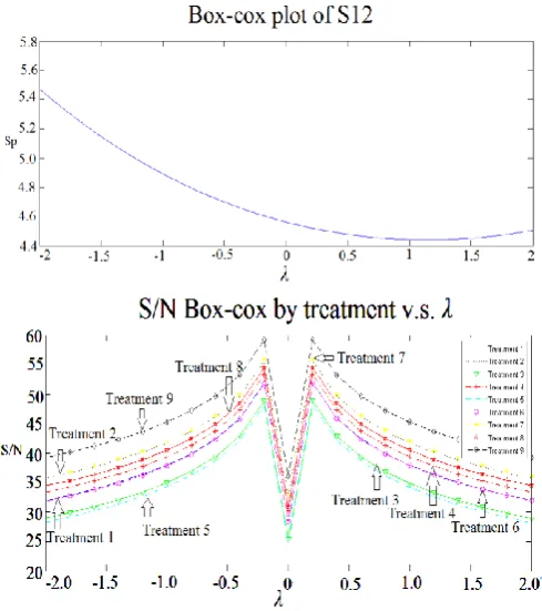
In addition, the transformed variables in all methods are determined the optimum. It is shown that the optimal λ level for BC is -0.28 for all cases. In the same way, the optimal δ level for DP is also -0.81 in all case. Moreover, the optimal
Ω level for AS is 500 for the smaller-the-better and the larger-the-better cases and 32.72 for the target-the-better case (Fig. 5). The optimal Ω level of LG is 500 for smaller-the-better and larger-smaller-the-better cases and 124.18 for the target-the-better case (Fig.6). Eventually, the optimal β level for PB is 1000 for the smaller-the-better and the larger-the-better cases and 124.18 for the target-the-larger-the-better case (Fig. 7).
[image:5.595.59.279.398.763.2]Fig. 5. Optimal Ω Level for AS for the Target-the-Better Case.
[image:5.595.307.552.455.594.2]Fig. 6. Optimal Ω Level for LG for the Target-the-Better Case.
Fig. 7. Optimal β Level for PB for the Target-the-Better Case. Case Data λ , Ω, Ω,δ, β Ranking Result
1 2 3 4
Smaller-the-better
N 1.00 C
BC -0.28 C A D
AS 500 C
LG 500 C A D
DP -0.81 C
PB 1000 C
Larger-the-better
N 1.00 C A D
BC -0.28 C
AS 500 C A D
LG 500 C
DP -0.81 C A D
PB 1000 C
Target-the-better (S/N)
N 1.00 C A B D
BC -0.28 C A B D
AS 37.32 C B A D
LG 124.18 C
DP -0.81 C A B D
PB 25.74 C B A D
Target-the-better (ANOM)
N 1.00 C D A B
BC -0.28 C A D
AS 37.32 C
LG 124.18 C
DP -0.81 C D A
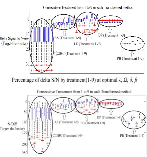
[image:5.595.309.552.633.770.2]After running 100 replicated experimental results from Matlab program to measure accuracy and distribution of results from each case, it is shown capability of each transformed method that Dual-power (DP) transformation has a lowest difference of signal-to-noise (central tendency). Arcsine (AS) and Logit (LG) transformation have a lower difference of signal-to-noise than Box-Cox (BC) transformation. Moreover, Parabolic (PB) transformation also have highest different of signal-to-noise among all transformed methods (Fig 8).
Fig 8. Comparative S/N Differences between Coded and Natural Data in case of Target-the-better.
VI. CONCLUSION
From all experimental results, In case of Taguchi orthogonal array without noise factors, performance measures of transformation methods are summarised that there are no transformed methods have the same result as natural data.it is ambiguous to speculate performance of each transformed methods. However, in another case, it is concluded that Dual-power transformation has a higher capability than the rest of methods because its result of experiments is most similar to natural data in all case and differences of signal-to-noise is more central tendency than the others. Arcsine transformation provides good result of transformed data in case of smaller-the-better and larger-the-better. On the other hand, Box-Cox transformation has only a good result in case of target-the-better. When considering to both of table and comparative graph, Arcsine seem to be better than Box-Cox. Furthermore, Logit and Parabolic do not have the same results as natural data in all cases. Logit seems to be slightly superior when compared to Parabolic based on signal-to-noise differences. Among them, researchers prefer Dual-power as the most appropriate method to transform data, at least in term of Taguchi orthogonal array with and without noise factors which are defined in specific case.
ACKNOWLEDGMENT
The authors wish to thank the Faculty of Engineering, Thammasat University, Thailand for the financial support.
REFERENCES
[1] Taguchi, G. and Konishi, S. Taguchi Methods, Orthogonal Arrays and Linear Graphs, Tools for Quality American Supplier Institute, American Supplier Institute, 1987, pp. 8-35.
[2] Taguchi G. Introduction to quality engineering, (Asian Productivity Organisation, Tokyo, 1990.
[3] Athreya, S. and Venkatesh, Y.D. Application of Taguchi Method for Optimisation of Process Parameters in Improving the Surface Roughness of Lathe Facing Operation, Vol. 1, Issue 7, International Refereed Journal of Engineering and Science (IRJES) 2012, pp. 13-19.
[4] Box, G.E.P. and Cox D.R. An Analysis of Transformation. Journal of the Royal Statistical Society. Series B (Methodological), Vol. 26, No.2, 1964, pp. 211-252.
[5] Osborne, J.W. Improving your Data Transformation: Applying Box-Cox Transformation, Practical Assessment, Research & Evaluation, Vol. 15, No.12, 2010, pp. 1531-7714.
[6] Duran, M.J. The Use of the Arcsine Transformation in the Analysis of Variance when Data Follow a Binomial Distribution. Master Thesis, State Univ. of New York, College of Environmental Science and Forestry Syracuse, New York, 1997.
[7] Raphael Guttargo, Andrian Raftery, Bayesian robust transformation and variable selection: a unified approach, The Canadian Journal of Statistics, Vol.37 No. 3 2009, pp. 361-380.
[8] Cordeiro, G.M. and Andrade, M.G. Transformed Symmetric Models. International Journal of Statistical Modelling, Vol. 11, No. 4, 2011 pp. 1-13.
[9] Motorcu, A.R. The Optimisation of Machining Parameters Using the Taguchi Method for Surface Roughness of AISI 8660 Hardened Alloy Steel, Strojniški vestnik Journal of Mechanical Engineering, 2010, pp. 391-401.
[10] Nalbant, M., Gökkaya, H. and Sur, G. Application of Taguchi method in the optimisation of cutting parameters for surface roughness in turning. Materials and Design, Vol. 28, 2010, pp. 1379-1385. [11] Raghu N. Kacker, R.N., Lagergren, E.S. and Filliben, J.J. Journal of
Research of the National Institute of Standards and Technology, Taguchi Vs Orthogonal Arrays are Classical Designs of Experiments, Vol. 96, No. 5, 1991.
[12] Chortirat, T., Chomtee, B. and Sinsomboonthong, J. (2011). Comparison of Four Data Transformation Methods for Weibull Distributed Data. Kasetsart J. (Nat. Sci.), Vol .18, No. 45, pp. 366-383.
[13] Luangpaiboon, P. and Chinda, K. (2014) Computer-based management of interactive data transformation systems using Taguchi’s robust parameter design, International Journal of Computer Integrated Manufacturing, DOI: 10.1080/0951192X.2014.941940. [14] Yang, Z. A Modified Family of Power Transformations. Economics