2
Original article
3
Use of posterior predictive assessments to evaluate model
4
fit in multilevel logistic regression
5
Martin J. G
REEN1,2*, Graham F. M
EDLEY3, William J. B
ROWNE46
7 1
School of Veterinary Medicine and Science, University of Nottingham, Sutton Bonington Campus,
8 Sutton Bonington, LE12 5RD, United Kingdom
9 2
School of Mathematical Sciences, University of Nottingham, Nottingham, NG7 2RD, United Kingdom
10 3
Department of Biological Sciences, University of Warwick, Coventry, CV4 7AL, United Kingdom
11 4
Department of Clinical Veterinary Science, University of Bristol, Langford House, Langford, Bristol,
12 BS40 5DT, United Kingdom
13 (Received 5 November 2008; accepted 24 March 2009)
14 Abstract –Assessing the fit of a model is an important final step in any statistical analysis, but this is
15 not straightforward when complex discrete response models are used. Cross validation and posterior
16 predictions have been suggested as methods to aid model criticism. In this paper a comparison is
17 made between four methods of model predictive assessment in the context of a three level logistic
18 regression model for clinical mastitis in dairy cattle; cross validation, a prediction using the full
19 posterior predictive distribution and two‘mixed’ predictive methods that incorporate higher level
20 random effects simulated from the underlying model distribution. Cross validation is considered a
21 gold standard method but is computationally intensive and thus a comparison is made between
22 posterior predictive assessments and cross validation. The analyses revealed that mixed prediction
23 methods produced results close to cross validation whilst the full posterior predictive assessment gave
24 predictions that were over-optimistic (closer to the observed disease rates) compared with cross
25 validation. A mixed prediction method that simulated random effects from both higher levels was
26 best at identifying the outlying level two (farm-year) units of interest. It is concluded that this mixed
27 prediction method, simulating random effects from both higher levels, is straightforward and may be
28 of value in model criticism of multilevel logistic regression, a technique commonly used for animal
29 health data with a hierarchical structure.
30 model fit / posterior predictive assessment / mixed predictive assessment / cross validation / Bayesian 31 multilevel model
32
33 1. INTRODUCTION
34 Random effect statistical models are being 35 increasingly used in veterinary sciences within 36 both frequentist and Bayesian frameworks. 37 Models are commonly specified with a binary 38 outcome to represent, for example, ‘diseased’
39 or ‘non-diseased’ states and therefore take the
40 form of multilevel logistic regression [5]. An
41 important element of constructing and finalising
42 a statistical model is to critically assess the fit
43 and performance of the model [8]. However,
44 model checking with discrete data regressions
45 is problematic because usual methods, such as
46 residual plots, have complicated reference
dis-47 tributions that depend on the parameters in the
48 model [7, 4]. Thus, these traditional methods
This is an Open Access article distributed under the terms of the Creative Commons Attribution-Noncommercial License
*
Corresponding author: martin.green@nottingham. ac.uk
1 are considered to be of limited value in discrete 2 outcome, random effects models [2]. It may be 3 because of this that, in the applied literature, 4 particularly when complex discrete response 5 models are specified, attention to model fit is 6 often cursory.
7 In this research, a recently reported method 8 of mixed predictive model assessment [10] is 9 examined and illustrated in the context of an 10 example from veterinary epidemiology. The 11 concept is extended from the two level Poisson 12 regression originally reported, to a three logistic 13 regression setting with the focus of interest on 14 prediction of bovine clinical mastitis on dairy 15 farms in a specific year [6].
16 Posterior prediction is a general term used 17 when data are generated under a proposed 18 model, often so that comparisons can be made 19 between specific features of the observed and 20 generated data [3]. The approach provides a 21 useful means for model assessment and cross 22 validatory posterior predictive distributions are 23 generally considered a ‘gold standard’ [10, 24 13]. Using cross validation, the data are parti-25 tioned ‘k’ times into subsets and an analysis is 26 initially performed on the ‘training’ subset. 27 The other ‘testing’ subset(s) are retained to val-28 idate the initial analysis by making predictions 29 from the data. Data predictions are compared 30 with the observed data. The procedure is 31 repeatedktimes andkmay equal the total num-32 ber of data points in the dataset or may repre-33 sent groups of data within the full set. An 34 important element of cross validation is that 35 predictions made on each subset of testing data 36 are independent of the observed outcome for 37 that subset. The comparisons are used to iden-38 tify discrepancies between model and data. 39 There is an important difference between 40 conventional residual analysis and cross valida-41 tion as a means of assessing outlying data 42 regions in the context of model assessment. In 43 conventional residual analysis, all data points 44 are included in the model fit and thus will have 45 a direct effect on model parameters and fitted 46 values, and hence the difference between 47 observed and fitted values. This is not the case 48 with cross validation when the data points or 49 groups have no influence at all on their cross 50 validatory predicted values, because they are
51 omitted during estimation, and in this respect,
52 classical residual plots are likely to be
over-53 optimistic in the assessment of model fit (i.e.
54 they may not identify all of the true outlying
55 regions) compared with cross validation.
Outly-56 ing units from cross validation are those for
57 which the other units do not provide sufficient
58 information for the model to fit; outliers from
59 residual analysis are those for which their
60 own influence is insufficient to provide a fit.
61 Therefore, regions of poor fit identified by cross
62 validation will not necessarily be identified by
63 residual analysis indicating the importance of
64 the former method.
65 A significant disadvantage of cross
valida-66 tion is that it is computationally intensive and
67 thus time consuming. A model has to be
re-68 estimated for each of k subsets and this may
69 include hundreds or thousands of data points
70 or regions. If Markov chain Monte Carlo
71 (MCMC) procedures are being used (as has
72 been recommended for random effects logistic
73 regression models [1]), and particularly with
74 large data sets, the timescale required means
75 that cross-validation may often become
imprac-76 tical (depending on the choice ofk).
77 Alternative methods to cross-validatory
pre-78 dictions have been suggested that have the
79 advantage of being more straightforward to
80 compute and less computationally intensive.
81 Gelman et al. [3] proposed use of the full model
82 predictive distribution to make predictions on
83 any required aspect of the data. This method
84 may be over-optimistic in the context of model
85 checking (i.e. it may fail to identify true
outly-86 ing regions) compared to cross-validation
87 because, as for residual analysis, the prediction
88 of any data region tends to be strongly
influ-89 enced by the equivalent observed data for the
90 region. Marshall and Spiegelhalter [10]
pro-91 posed a method termed the ‘mixed’ predictive
92 check which they have illustrated in the context
93 of disease mapping, and which appeared to
per-94 form in a similar manner to cross validation.
95 The mixed predictive check incorporates
simu-96 lated random effects, generated from their
97 underlying distribution which is characterised
98 from fitting the initial model, rather than the
99 random effects estimated directly from the data.
1 also been reported in the context of differential 2 gene expression [9]. In that study, mixed pre-3 dictive Markov chain P values were used to 4 evaluate hierarchical models [3, 10] but com-5 parisons were not made between different meth-6 ods of posterior predictions as a means to assess 7 model fit. In this context, Markov chainP val-8 ues are an indicator of the probability that a pre-9 dicted data region is numerically higher 10 (or lower) than the observed equivalent. If the 11 probability is high (typically greater than 95% 12 or 97.5%) or low (typically less than 5% or 13 2.5%) then it suggests that the model is per-14 forming poorly in the data region.
15 The purpose of this paper is to illustrate and 16 compare four methods of model predictive 17 assessment in the context of a multilevel logis-18 tic regression model, in which the specific clin-19 ical interest was the prediction of disease in a 20 higher level unit (in this example a farm-year). 21 The methods are cross validation, a full poster-22 ior predictive assessment and two mixed predic-23 tive methods based on the approach proposed 24 by Marshall and Spiegelhalter [10]. An exten-25 sion to the concept of the mixed prediction is 26 described that is generalisable to three level 27 hierarchical models.
28 2. MATERIALS AND METHODS
29 2.1. The data and initial model
30 The data for this analysis comprises clinical
mas-31 titis and farm management information from fifty two
32 commercial dairy herds, located throughout England
33 and Wales, with a mean herd size of approximately
34 150 cows and has been described in detail previously
35 [6]. Data were collected over a two year period. The
36 aim of the original research was to investigate the
37 influence of cow characteristics, farm facilities and
38 herd management strategies during the dry period,
39 on the rate of clinical mastitis after calving. Interest
40 was focussed on identifying determinants for clinical
41 mastitis occurrence and to assess the extent to which
42 these determinants could be used to predict the
occur-43 rence of clinical mastitis in each year on each farm.
44 The response variable was at the cow level; a cow
45 either got a case of clinical mastitis (= 1) or not
46 (= 0) within 30 days of calving and a cow could be
47 at risk in both years of the study. Predictor variables
48
were included at the cow, year and farm levels. The
49
model hierarchical structure was cows within
farm-50
years within farms, and can be summarised as:
CMijkBernouilliðpijkÞ
LogitðpijkÞ ¼b0þb1X
ð1Þ ijkþb2X
ð2Þ jk
þb3Xðk3Þþujkþv0kþv1kPijk
ujkNð0;r2uÞ;vk¼ v0k
v1k !
MVNð0;XvÞ
ð1Þ 5252
53
where the subscripts i, j and k denote the three
54
model levels, pijkthe fitted probability of clinical
55
mastitis (CM) for cow i in year j on farm k, b0 56
the regression intercept,Xðijk1Þ the vector of
covari-57
ates at cow level,b1the coefficients for covariates 58
Xðijk1Þ,Xðjk2Þ the vector of farm-year level covariates,
59
b2the coefficients for covariatesX
ð2Þ jk ,X
ð3Þ k the
vec-60
tor of farm level covariates,b3the coefficients for 61
covariatesXðk3Þ,Pijkis a covariate (withinX ð1Þ ijk) that
62
identifies cows of parity one (after first calf),ujkis a
63
random effect to reflect residual variation between
64
years within farms, and v0k and v1k are random
65
effects to reflect residual variation between farms,
66
and for the difference in rates for parity 1 cows
67
between farms respectively.
68
Model selection was made from a rich dataset of
69
more than 350 covariates. Model building has been
70
described in detail previously [6] but briefly
pro-71
ceeded as follows. Each of the covariates was
exam-72
ined individually, within the specified model
73
framework, to investigate individual associations with
74
clinical mastitis whilst accounting for the data
struc-75
ture. Initial covariate assessment was carried out using
76
penalised quasi-likelihood for parameter estimation
77
(MLwiN, [11]) and final models were selected using
78
MCMC for parameter estimation in WinBUGS [12].
79
A burn-in of at least 2 000 iterations was used for
80
all MCMC runs during which time model
conver-81
gence had occurred. Parameter estimates were based
82
on a further 8 000 iterations. The final model included
83
the following predictor variables; cow parity, cow
his-84
toric infection status, whether the farm maintained a
85
cow standing time of 30 min after administration of
86
treatments at drying off (the end of the previous
lacta-87
tion), whether farms reduced the milk yield of high
88
yielding cows before drying off, whether cow bedding
89
was disinfected during the early dry period, type of
90
cow bedding during the late dry period, the time
per-91
iod between sequential cleaning out of the calving
92
pens, and the time between calving and the cows
93
1 2.2. Predictive assessments
2 Of particular clinical interest in the research was the
3 prediction of the incidence rate of clinical mastitis
4 (number of cases per cow at risk) for each of thej=
5 1. . .103 farm-years and thus the predictions of these
6 rates were used to investigate methods of model
assess-7 ment. Four methods of predictive assessment were
8 compared; cross validation, a full posterior predictive
9 check and two ‘mixed’ predictive assessments similar
10 to that suggested by Marshall and Spiegelhalter [10].
11 After final model selection, each method of prediction
12 was incorporated into the MCMC process. At each
iter-13 ation after model convergence, a prediction was made
14 for the occurrence of mastitis for each individual cow
15 (yijk) by drawing from the appropriate conditional
16 probability distribution (see below). Similarly, at each
17 iteration, the number of predicted cases of clinical
mas-18 titis were summed over all cows in each farm-year and
19 divided by the total cows at risk in each farm-year, to
20 provide an MCMC estimate of the farm-year incidence
21 rate of clinical mastitis. Predictions were made from 8
22 000 MCMC iterations after model convergence.
23 To describe the four methods of predictive
assess-24 ment, we condense the model terms, such that the
25 disease status for each cow (yijk) is conditional on a
26 set of model fixed effect parameters b, covariates 27 (at various levels)Xijk, and random effectsvk, andujk:
yijkp yijkjb;Xijk;Vk;Ujk
29 29
3031 The random effects have parameters represented 32 byr2
u andXv.
Ujkp Ujkjr2u
Vkp Vð kjXVÞ 34
34
3536 The four methods of predictive assessment
37 employed were:
38 A. Cross validation (‘‘xval’’). Each of the 103
39 farm-years was removed from the analysis
40 in turn and the model fitted to a reduced
41 data set excluding the jkth farm-year
42 (denoted (jk)), from which new model
43 parameters were estimated ðbðjkÞ; vðjkÞ;
44 uðjkÞ; r2
u jk ð Þ
; XvðjkÞÞ:A replicate
obser-45 vation for the omitted data,yijkxvalwas simu-46 lated from the conditional distribution;
yijkxvalp yijkxval
bðjkÞ
;Xijk; ujkxval;vkxvalÞ ujkxvalp ujkxval
r2 u
jk ð Þ
Þ vkxvalp vð kxvaljXvðjkÞÞ
ð2Þ
48 48
49
B. Posterior predictive assessment from the full
50
data (‘‘full’’). The predictive distribution was
51
conditional on all fixed effect and random
52
effect parameters estimated in the final
53
model and a replicate observationyijkfull
gen-54
erated from the conditional distribution;
yijkfullp y ijk
full
b;Xijk;vk;ujkÞ ð3Þ 5656 57
C. Mixed prediction 1 (‘‘mix1’’). This
predic-58
tive distribution was conditional on the fixed
59
effect parameters and the random effect
dis-60
tributions from which new random effects,
61
ujkmix1 and vkmix1, were simulated to make
62
the prediction. Thus a replicate observation
63
yijkmix1 was generated from the conditional
64
distribution;
yjkmix1p yjkmix1
b;Xijk;ujkmix1
;vkmix1Þ
ujmix1p ujkmix1
r2 uÞ vkmix1p vð kmix1jXvÞ
ð4Þ
66 66 67
D. Mixed prediction 2 (‘‘mix2’’). This
predic-68
tive distribution was conditional on the fixed
69
effect parameters, the random effects
distri-70
bution at level 2, (from which new random
71
effects,ujkmix2were simulated), and the level
72
3 random effects from the model,vk. Thus a
73
replicate observation yijkmix2 was simulated
74
from the conditional distribution;
yijkmix2p yijkmix2
b;Xijk;ujkmix2;vkÞ
ujkmix2p ujkmix2
r2 uÞ
ð5Þ
76 76 77 78 2.3. Comparisons between methods
79 of predictive assessments
80
In each case, predictions of farm-year incidence
81
rates of clinical mastitis were compared with
82
observed rates. Predictions from cross validation
83
(taken as a gold standard) were also compared to
84
the other methods of prediction to assess which best
85
mimicked this procedure. To assess the degree of
dis-86
crepancy between observed and predicted farm-year
87
incidence rate of mastitis, the predicted distributions,
88
yjkpred were compared to the observed values using 89
Monte Carlo predictiveP values. At each iteration
90
of the MCMC procedure, an indicator variable was
91
set to 1 when yjkpred>y
jk, to 0.5 if yjkpred¼yjk 92
and to 0 if yjkpred<y
jk; the Monte CarloP value 93
1 Therefore predictiveP values > 0.975 or < 0.025
2 indicated that the probability of the observed
inci-3 dence rate of clinical mastitis being within the
pre-4 dicted distribution was less than 5% and
5 represented a relatively extreme result.
6 3. RESULTS
7 Figure 1 (A–D) illustrates the mean pre-8 dicted incidence rate of clinical mastitis for each 9 method of posterior prediction, plotted against 10 the observed incidence of clinical mastitis. 11 The graphs illustrate that the full posterior pre-12 dictive method most closely resembled the
13 observed data and cross validation and the
14 ‘‘mix1’’ method displayed considerably more
15 variability. The ‘‘mix2’’ method provided an
16 intermediate result. Figure 2 illustrates the
com-17 parison between mixed and full predictive
18 methods and cross validation. Both mixed
pre-19 dictive methods yielded better estimates of the
20 cross validatory prediction than the full
poster-21 ior predictive method, and the ‘‘mix2’’ method
22 produced estimates most similar to cross
23 validation.
24 The median error for each predictive method
25 was calculated as the median of the unsigned
dif-26 ferences between predicted and cross validatory
27 farm-year incidence rates of clinical mastitis, as
A. Cross validation -r2 = 42.4 %
0 0.1 0.2 0.3 0.4 0.5
0 0.1 0.2 0.3 0.4 0.5 Predicted Incidence Rate of Mastitis (cross validation)
Observed Incidence Rate of Mastitis
B. Full predictive method -r2 = 85.8%
0 0.1 0.2 0.3 0.4 0.5
0 0.1 0.2 0.3 0.4 0.5 Predicted Incidence Rate of Mastitis (full posterior
prediction)
Observed Incidence Rate of Mastitis
C. Mixed prediction method 1 -r2 = 44.4%
0 0.1 0.2 0.3 0.4 0.5
0 0.1 0.2 0.3 0.4 0.5 Predicted Incidence Rate of Mastitis (mix prediction 1)
Observed Incidence Rate of Mastitis
D. Mixed prediction method 2 -r2 = 74.2%
0 0.1 0.2 0.3 0.4 0.5
0 0.1 0.2 0.3 0.4 0.5 Predicted Incidence Rate of Mastitis (mix prediction 2)
[image:5.468.58.427.64.391.2]Observed Incidence Rate of Mastitis
1 a percentage of the cross validatory farm-year 2 incidence rate of clinical mastitis. The median 3 errors were 13.7%, 11.5% and 9.4% for the full 4 posterior prediction, the mixed prediction 1, 5 and for mixed prediction 2 respectively.
[image:6.468.233.418.68.508.2]6 Figure 3 illustrates the MCMC P values
7 obtained from the different predictive methods
8 to compare with the most extreme P values A – Full predictive method -r2 = 71.5
0 0.1 0.2 0.3 0.4 0.5
0 0.1 0.2 0.3 0.4 0.5 Predicted Incidence Rate of Mastitis (full) Predicted Incidence Rate of Mastitis (cros validation)
B – Mixed prediction method 1 -r2 = 78.6%
0 0.1 0.2 0.3 0.4 0.5
0 0.1 0.2 0.3 0.4 0.5 Predicted Incidence Rate of Mastitis (mixed prediction 1) Predicted Incidence Rate of Mastitis (cros validation)
C – Mixed prediction method 2 -r2 = 84.3%
0 0.1 0.2 0.3 0.4 0.5
0 0.1 0.2 0.3 0.4 0.5 Predicted Incidence Rate of Mastitis (mixed prediction 2) Predicted Incidence Rate of Mastitis (cros validation)
Figure 2. Plots of cross validatory predictions of farm-year clinical mastitis incidence against full and mixed predictive methods of farm-year clinical mastitis incidence (cases per cow at risk per year).
A – Full predictive method.
0 0.1 0.2 0.3 0.4 0.5 0.6 0.7 0.8 0.9 1
0 0.1 0.2 0.3 0.4 0.5 0.6 0.7 0.8 0.9 1
MCMC P value (full posterior prediction)
MCMC P value (cross validation)
B – Mixed prediction method 1
0 0.1 0.2 0.3 0.4 0.5 0.6 0.7 0.8 0.9 1
0 0.1 0.2 0.3 0.4 0.5 0.6 0.7 0.8 0.9 1
MCMC P value (mixed prediction 1)
MCMC P value (cross validation)
C – Mixed prediction method 2.
0 0.1 0.2 0.3 0.4 0.5 0.6 0.7 0.8 0.9 1
0 0.1 0.2 0.3 0.4 0.5 0.6 0.7 0.8 0.9 1
MCMC P value (mix prediction 2)
[image:6.468.36.212.72.345.2] [image:6.468.35.214.354.485.2]MCMC P value (cross validation)
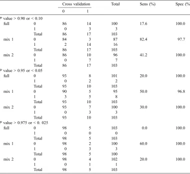
1 identified with cross validation, these being the 2 most divergent regions eligible for identification 3 and further investigation. At large and smallP 4 values (P < 0.20 or > 0.80) the mixed predic-5 tive methods performed more similarly to cross 6 validation than the full posterior prediction with 7 the ‘‘mix1’’ method most closely representing 8 cross validatory MCMCPvalues. This is con-9 firmed in Table I that provide the sensitivity and 10 specificity for each predictive method, taking 11 cross validation MCMCPvalues as the ‘‘gold 12 standard’’, and different P value thresholds.
13 The ‘‘mix1’’ method had the highest sensitivity
14 indicating that this method identified the largest
15 proportion of ‘‘true’’ extreme values as
deter-16 mined by cross validation. The ‘‘mix1’’ method
17 identified 82.4% (14 out of 17) of extreme
val-18 ues when a threshold of < 0.10 or > 0.90 was
19 used and 60% (3 out of 5) of extreme values
20 with a threshold set at < 0.025 or > 0.975.
21 The computing times to complete 10 000
22 iterations (using an Intel Centrino 2.0 GHz
Pro-23 cessor, 1.5GB RAM) for 103 cross validatory
[image:7.468.53.433.109.458.2]24 predictions and the ‘‘mix1’’ method were 334 Table I.Sensitivity and specificity of MCMCPvalues for each prediction method (full = full posterior predictive method, mix 1 and mix 2 = mixed predictive methods 1 and 2 respectively) compared to MCMC Pvalues for cross validation, at differentPvalue thresholds (as specified).
Cross validation Total Sens (%) Spec (%)
0 1
Pvalue > 0.90 or < 0.10
full 0 86 14 100 17.6 100.0
1 0 3 3
Total 86 17 103
mix 1 0 84 3 87 82.4 97.7
1 2 14 16
Total 86 17 103
mix 2 0 86 10 96 41.2 100.0
1 0 7 7
Total 86 17 103
Pvalue > 0.95 or < 0.05
full 0 93 8 101 20.0 100.0
1 0 2 2
Total 93 10 103
mix 1 0 90 5 95 50.0 96.8
1 3 5 8
Total 93 10 103
mix 2 0 93 7 100 30.0 100.0
1 0 3 3
Total 93 10 103
Pvalue > 0.975 or < 0. 025
full 0 98 5 103 0.0 100.0
1 0 0 0
Total 98 5 103
mix 1 0 98 2 100 60.0 100.0
1 0 3 3
Total 98 5 100
mix 2 0 98 4 102 20.0 100.0
1 0 1 1
1 h and 3.6 h respectively. This did not include the 2 time required to format the data and set up each 3 model and this took approximately the same 4 time per model. Thus it took approximately 5 103 times longer for the cross validatory predic-6 tions than the ‘‘mix1’’ method.
7 4. DISCUSSION
8 Identifying divergent data regions in statisti-9 cal modelling is important for two reasons. 10 Firstly, numerous divergent regions could indi-11 cate that underlying statistical assumptions are 12 incorrect, for example the model does not cap-13 ture the true data structure. Secondly, individual 14 divergent units could represent those that are 15 fundamentally different from other units in the 16 dataset after accounting for predictor variables, 17 and the possible absence of unknown but 18 important explanatory covariates. In either case, 19 further investigations would be warranted. 20 Cross validation provides a useful method of 21 accurately identifying divergent units in com-22 plex statistical models, but faster methods 23 would be of practical value in model assess-24 ment and it was for this reason that the alterna-25 tive strategies were investigated in this research. 26 The predictions of clinical mastitis incidence 27 rates obtained from the different methods show 28 clear differences in results obtained, as shown 29 in Figure 1. The full predictive method pro-30 vided predicted incidence rates of clinical mas-31 titis that most closely resembled the observed 32 incidence rates, but these appeared to be over-33 optimistic in terms of model performance in 34 comparison to cross validatory predictions. This 35 is not surprising since the random effects from 36 the initial model are directly incorporated into 37 the prediction steps but it does highlight the dif-38 ference between this method and cross 39 validation.
40 For the three level logistic regression models 41 in this example, the mixed predictive methods 42 provided a better approximation to cross-43 validation than the full posterior predictive 44 assessment. This is concordant with the first 45 study that used a mixed prediction for approxi-46 mating cross validation in a two level Poisson 47 model for disease mapping [10]. In the current
48 study using a three level logistic regression
49 model, the ‘‘mix2’’ method provided the closest
50 overall approximation to cross validatory
pre-51 dictions of farm-year incidence of clinical
52 mastitis. However, the ‘‘mix1’’ method
per-53 formed best for the more extreme outlying
val-54 ues identified by cross validation and thus this
55 method was more useful for identifying the
56 most divergent higher level units in these data.
57 The mixed predictive methods look promising
58 as a means of practical model assessment for
59 the relatively common statistical approach of
60 multilevel logistic regression and as such,
war-61 rant further investigations.
62 Importantly, the mixed predictive methods
63 take considerably less time to implement
64 (in this example approximately one hundredth
65 of the time of cross validation) and therefore
pro-66 vide a clear advantage in terms of practical use.
67 The ‘‘mix2’’ method is essentially a compromise
68 between the ‘‘mix1’’ method and a full posterior
69 prediction. The method simulates a new random
70 effect at level 2 but uses the estimated random
71 effects from the model at level 3. In the current
72 example there were only two level 2 units for
73 each level 3 unit and it may be that if more level
74 two units existed for each level 3 units, mixed
75 prediction method 2 would tend to become
sim-76 ilar to mixed method 1 (the higher level unit
hav-77 ing less influence on the predicted data).
78 Similarly, the relative performance of the two
79 mixed predictive methods may depend on the
80 relative sizes of the higher level variances and
81 more research into the importance of the relative
82 size of higher level variances when using mixed
83 predictive methods would be beneficial. In this
84 example the variance at level two (farm-year)
85 was 0.06 and at level three (farm) was 0.10
86 (for cows greater than parity one) and 0.64 (for
87 cows of parity one). If the level three variances
88 had been very small in comparison to the level
89 2 variance, it is possible that both mixed
predic-90 tive methods used in this study would have
91 yielded similar results. Further investigations
92 of mixed predictive methods using different
93 types of models, numbers of levels, units per
94 level and relative sizes of higher unit variances
95 would be worthwhile.
96 From our results, it would appear that, out of
1 likely to provide the closest representation of 2 cross validation for potentially divergent data 3 regions in multilevel logistic regression. How-4 ever, it is important to note that these results 5 apply only to one dataset and whilst in agree-6 ment with a previous study [10], need to be 7 viewed with this perspective. It may be possible 8 to generalise this approach to logistic regression 9 and other multilevel models, but more research 10 in this area is required.
11 Our results indicate that whilst mixed predic-12 tions provide a reasonable approximation to 13 cross validation, they do not provide precise 14 replication of the results. Therefore, a pragmatic 15 approach for implementation of mixed predic-16 tive assessments may be for an initial highlight-17 ing of possible divergent data regions on which 18 to undertake further model checking using cross 19 validation. Thus, instead of undertaking cross 20 validation on all possible regions an intermedi-21 ate step could be to first use a mixed prediction 22 approach and then to use cross validation for 23 data regions that are potentially divergent based 24 on the mixed prediction. A reduced mixed pre-25 diction MCMCPvalue threshold could be used 26 to improve the likelihood that all ‘true’ outliers 27 are identified, possibly the central 80 percentile 28 region and cross validation then carried out on 29 regions that fall outside this interval. This 30 would increase the sensitivity of identifying 31 ‘‘true’’ divergent regions using the mixed meth-32 ods but would reduce the computing time 33 required compared to using cross validation 34 for all regions.
35 Assessment of model performance is impor-36 tant and problematic particularly when large 37 datasets and complex model structures are used. 38 Posterior predictions are recognised as a useful 39 method to investigate model fit and more 40 research on mixed posterior predictions may 41 be useful to facilitate straightforward, fast 42 assessments for these types of model.
43 Acknowledgements. Martin Green is funded by a
44 Wellcome Trust Intermediate Clinical Fellowship.
45 REFERENCES
46
[1] Browne W.J., Draper D., A comparison of
47
Bayesian and likelihood-based methods for fitting
48
multilevel models, Bayesian Analysis (2006) 1:
49
473–514.
50
[2] Dohoo I.R., Martin W., Stryhn H., Veterinary
51
epidemiologic research, Atlantic Veterinary College
52
Inc., Prince Edward Island, Canada, 2003.
53
[3] Gelman A., Meng X., Stern H., Posterior
predic-54
tive assessment of model fitness via realized
discrep-55
ancies, Statistica Sinica (1996) 6:733–807.
56
[4] Gelman A., Goegebeur Y., Tuerlinckx F., van
57
Mechelen I., Diagnostic checks for discreet data
58
regression models using posterior predictive
simula-59
tions, Appl. Stat. (2000) 49:247–268.
60
[5] Goldstein H., Multilevel Statistical Models,
61
London, Edward Arnold, 1995.
62
[6] Green M.J., Bradley A.J., Medley G.F., Browne
63
W.J., Cow, farm and management factors during the
64
dry period that determine the rate of clinical mastitis
65
after calving, J. Dairy Sci. (2007) 90:3764–3776.
66
[7] Landwehr J.M., Pregibon D., Shoemaker A.C.,
67
Graphical methods for assessing logistic regression
68
models (with discussion), J. Am. Stat. Assoc. (1984)
69
79:61–83.
70
[8] Langford I., Lewis T., Outliers in multilevel data,
71
J. R. Stat. Soc. Ser. A (1998) 161:121–160.
72
[9] Lewin A., Richardson S., Marshall C., Glazier A.,
73
Aitman T., Bayesian modelling of differential gene
74
expression, Biometrics (2006) 62:1–9.
75
[10] Marshall E.C., Spiegelhalter D.J., Approximate
76
cross-validatory predictive checks in disease mapping,
77
Stat. Med. (2003) 22:1649–1660.
78
[11] Rasbash J., Browne W.J., Healy M., Cameron B.,
79
Charlton C., MLwiN Version 2.02, Multilevel Models
80
Project, Centre for Multilevel Modelling, Bristol, UK,
81
2005.
82
[12] Spiegelhalter D.J., Thomas A., Best N.,
Win-83
BUGS Version 1.4.1., Imperial College and MRC,
84
UK, 2004.
85
[13] Stern H.H., Cressie N., Posterior predictive
86
model checks for disease mapping models, Stat.
87
Med. (2000) 19:2377–2397.