On the selection of connectivity based metrics for WSNs using a classification of application behaviour

On the Selection of Connectivity-based Metrics for WSNs using a Classification of

Application Behaviour

Alan W. F. Boyd, Dharini Balasubramaniam, Alan Dearle, Ron Morrison School of Computer Science, University of St Andrews

{alanb, dharini, al, ron}@cs.st-andrews.ac.uk

Abstract—This paper addresses a subset of Wireless Sensor Network (WSN) applications in which data is produced by a set of resource-constrained source nodes and forwarded to one or more sink nodes. The performance of such applications is affected by the connectivity of the WSN, since nodes must remain connected in order to transfer data from sources to sinks. Designers use metrics to measure and improve the efficacy of WSN applications. We aim to facilitate the choice of connectivity-based metrics by introducing a classification of WSN applications based on their data collection behaviour and indicating the metrics best suited to the evaluation of particular application classes. We argue that no suitable metric currently exists for a significant class of applications with the following characteristics: 1) application data is periodically routed or disseminated from source nodes to one or more sink nodes, and 2) the application can continue to function with the loss of source nodes although its useful network lifetime diminishes as a result. We present a new metric, known as Connectivity Weighted Transfer, which may be used to evaluate WSN applications with these characteristics.

Keywords-sensor networks; life estimation; system analysis and design

I. INTRODUCTION

A Wireless Sensor Network (WSN) may be considered as a collection of small, battery-operated, resource-constrained nodes, each containing a low power radio. The collection may include a number of:

1) source nodes, which typically contain sensors capable of measuring environmental factors such as tempera-ture or humidity, and may additionally act as interme-diate nodes (defined below),

2) sink nodes, which receive the data generated by the sources, and,

3) intermediate nodes, which aid the transmission of data from sources to sinks.

Due to the energy constraints of nodes, the efficacy of a WSN application is often measured in terms of network lifetime[1]. We limit our consideration in this paper touseful network lifetime, which reflects the duration for which a WSN is alive and functional according to a user-defined set of criteria, rather than merely alive. The criteria may include the requirements of a specific application as well as network assumptions and configurations.

Many WSN applications benefit from having data from a diversity of sources. For example, if the aim of an

application is to detect the boundary of a forest fire, increas-ing the number of sources may provide greater accuracy. However, doing so might cause sources that also act as intermediate nodes to quickly expire, leading to a reduction in the total data transferred as will be shown in Section IV-A. Application requirements determine whether such a reduction is an acceptable trade-off for increased diversity of data.

Application designers use metrics to measure and optimise their WSN deployments. The motivation for our work is to aid their choice of metrics by providing a mapping between suitable metrics and application classes based on data collection behaviour. For example, the selection of a routing protocol may improve (according to some metric) the application’s useful network lifetime. The choice of metric is important, since it must accurately reflect the duration for which the application remains useful. We have focused on connectivity-based metrics, since networks with a (source, sink) architecture only remain useful as long as the sources and sinks remain connected. A number of connectivity-based metrics that measure useful network lifetime have been described in the literature. We review the pertinent metrics from the comprehensive survey provided by Dietrich and Dressler in [1].

The contributions of this paper are twofold. Firstly, we define a set of characteristics that may be used to classify applications based on their data collection behaviour in order to provide a mapping that indicates which metric will yield the most appropriate measure of useful network lifetime for each WSN application class. We note that the reviewed metrics do not accurately reflect the useful network lifetime of applications that meet the following criteria:

• Data is periodically produced at several source nodes and either routed or disseminated through the network to one or more sink nodes.

• The application remains functional, although its useful-ness decreases, when source nodes expire.

II. WSNAPPLICATION DEPLOYMENTS

In this section, we discuss a number of WSN application deployments that feature prominently in the literature. The deployments discussed will form the basis of the application classification in Section III.

One of the best-known WSN deployments is the habitat monitoring of Great Duck Island (GDI) [2]. 150 source nodes were placed on the island and periodically routed data to a local gateway node (sink). The application was not dependent upon all sources being active; sources were shown to expire at various points during the 120-day deployment. ZebraNET [3] used a WSN to track the locations of zebras in Kenya. The deployment of nodes called for 30 specially built collars to be attached to zebras and act as source nodes. GPS data was periodically gathered and stored at each source. When a pair of sources came into contact, their data was shared. All data was disseminated through the network in this manner. Since the application gathered the positional data of each zebra, we infer that loss of individual sources would not cause the application to become unusable. However, the number of correlations between zebra positions would be reduced.

Wisden [4] is a proposed system for structural monitoring in which source nodes are manually placed on a structure, such as a bridge, to monitor vibration levels. The authors note that Wisden is data loss intolerant and therefore, all sources must remain active. Sources route data through the network to the sink and store it locally to prevent its loss.

CenseMe [5] is a social-networking WSN application, which is designed to operate on mobile phones. The ap-plication infers what a user is doing (and with whom) by means of the microphone, GPS receiver, accelerometer and bluetooth receiver. For example, the bluetooth receiver and accelerometer may allow the inference that the user is “walk-ing with Bob”. Simple conclusions (known as primitives) are uploaded to a database via GPRS or 802.11 where they can be analysed further. CenseMe was run by 22 users in its test deployment. Since users could simply switch their phones off at any time, it is concluded that CenseMe is capable of operating with source loss, albeit with reduced functionality. A system for analysing the microclimates surrounding redwood trees has been produced by Tolle [6]. In Tolle’s deployment, 33 source nodes were placed on a tree. Each source generated and stored periodic data based on temper-ature, humidity and radiation readings before routing it to a sink at the bottom of the tree. The application was resistant to source loss as it continued to operate despite a number of failures.

NAWMS [7] is a proposed system to provide fine granu-larity detail regarding water usage in homes. In NAWMS, the sink node is attached to the water meter. By automatically calibrating vibration levels of a pipe and the water travelling through the meter, the system can display water usage for

devices. It is estimated that a house with 3 bedrooms and 2 bathrooms may require 17-21 source nodes. All sources must remain active in order to perform calibration.

PermaSense [8] is a project that aims to gather envi-ronmental data regarding permafrost in the Alps for at least 3 years. Approximately 25 sources periodically gather environmental data, which is both stored and routed to a sink. The project has tight constraints regarding the loss of data; consequently, the failure of even a single source would render the application unusable.

Volcano monitoring [9] has been carried out by Werner-Allen at the Reventador volcano in Ecuador. Each of 16 source nodes buffered its last 20 minutes of sensor readings. Any event of interest detected by a source was reported to the sink. If the sink received several simultaneous events of interest, it would query all sources for their buffered data from the previous 60 seconds. A small number of sources were lost during the operation of the network, leading to the conclusion that the application remains operational with source node loss.

III. APPLICATION CLASSIFICATION

A novel classification of applications is now presented to facilitate the choice of metrics. Unlike existing work [10] [11], it considers the data collection behaviour of each application, which enables designers to choose a metric appropriate to the nature of the (source, sink) interaction. The following criteria are considered:

• action on data,

• data generation method, and

• resilience to source loss.

Action on data refers to the action taken by a source when it produces data. The source must eitherroute,disseminate or upload data. It may optionally also store, buffer or actuate. Routing refers to the forwarding of data, possibly through multiple hops, towards one or more destinations. Disseminating is the process in which data is flooded throughout the network to all nodes. Uploading sends the data directly from the source node to a sink without the source making any routing decisions. Since it is assumed that data is sent from sources to sinks, one of these three actions must take place. Of the remaining actions, storage refers to the process in which a source node records data on a local non-volatile medium for collection at a later date. Buffering involves the temporary storage of data for some (possibly undefined) period. Actuation refers to a physical action taken by the source, such as activating a motor.

the source responds to some external phenomena of interest as defined by the user.

The final criterion is that of resilience to source loss, which models the lifetime of the application as a function of source loss. The application may have no resilience to source loss. It may be able to tolerate the loss of a specific number of sources. The resilience may also beperformance dependent in which case the application’s usefulness de-pends on the number of sources remaining, thus requiring a high source diversity for as long as possible.

The classification of applications described in Section II using the above set of criteria can be found in Table I.

IV. COMMON METRICS

Dietrich and Dressler [1] have recently carried out a comprehensive review of metrics which are categorised into one of the following groups:

1) number of live nodes, 2) sensor coverage, 3) connectivity,

4) sensor coverage and connectivity,

5) application quality of service requirements, and, 6) triple of (connectivity, number of live nodes, coverage)

which is considered as “the definition provided by Blough and Santi” in [1].

In this paper, we are only concerned with those metrics that are connectivity-based. We therefore focus on those metrics that fall under categories 3, 4 and 6, all of which take connectivity into account:

1) total data transfer, which is considered a sub-category of connectivity in [1],

2) k-of-n lifetime, which is considered as a sub-category of number of live nodes and of connectivity in [1], 3) sink connectivity, which is covered as a metric of

connectivity in [1],

4) triple of (connectivity, number of live nodes, cover-age), and,

5) sensor coverage and connectivity. A. Total data transfer

Several authors have considered measuring lifetime in terms of the total data transferred by the network. Baydere [13] considers network lifetime “in terms of total messages transmitted”. Other authors consider a more general mea-surement, as in the case of Giridhar [14] who measures lifetime in terms of “the maximum number of times a certain data collection function or task can be carried out without any node running out of energy”.

An advantage of this metric is that it is possible to mea-sure the data transferred across a single node or in response to a specific event. Thus it is possible to measure the effect of an event or how specific nodes are used. However, the data transfer metric suffers from two disadvantages. Firstly, as reported by Dietrich and Dressler [1], it may be ineffective

where data aggregation occurs. Secondly, the metric may be of limited use in networks where sources forward data on behalf of other sources. These situations are discussed below:

Data aggregation is a technique intended to reduce energy expenditure in routing protocols. It combines data from multiple sources into a single, smaller piece of data. Since the data transfer metric only measures the quantity of data received by sink nodes and data aggregation reduces the amount of data transmitted, the metric does not accurately reflect the quantity of information received.

When sources forward data on behalf of other sources, they may expend more energy than they would if they had generated the data themselves. Consequently, to reduce the energy consumption of sources, the optimal solution is for sources to refuse to forward data that originates elsewhere. However, this approach may lead to a loss of source diversity, since some sources may be unable to send their data towards a sink. We refer to this as the source forwarding problem. Attempting to increase source diversity by forcing sources to forward all data may be insufficient. A poor application or routing protocol may cause sources that rely on source forwarding to expire. Thus, the application may appear to be near optimal according to the data transfer metric even though the source diversity would be reduced.

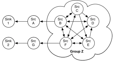
For example, consider a scenario in which the inefficient maximum-hop routing protocol is employed within the net-work shown in Figure 1. The netnet-work consists of nine nodes, including two sinks and seven sources (A-G). A subset of sources B-F is referred to as group Z for convenience. The source nodes generate data and send it towards one of the sink nodes. A directed edge from a node X to a node Y indicates that Y receives every transmission made by X. Note that not all edges are bidirectional.

Sink 1

Src A

Src C

Src B

Src F

Src D

Src E

Group Z

Src G Sink

2

Figure 1. An example network in which maximum hop routing is applied

Table I

CLASSIFICATION OF APPLICATIONS

Application Nodes Sources Sinks Action on data Generation Resilience

GDI 152 150 2 Route Periodic Performance dependent

ZebraNET 31 30 1 Disseminate Periodic Performance dependent

Wisden Tens Tens 1 Route/store Event No

CenseMe 23 22 1 Upload Periodic Performance dependent

Redwoods 34 33 1 Route/store Periodic Performance dependent

NAWMS 18-22 17-21 1 Upload/actuate Periodic No

PermaSense 26 25 1 Route/store Periodic No

Volcano 17 16 1 Route/buffer Event/query Performance dependent

Consequently, any data generated by a node in Z will be transmitted and received five times before it reaches either A or G. Every transmission made by a source in Z is overheard by sources B and F, which connect Z to the sinks. Thus, every piece of data generated by a node in Z will be received/overheard four times and transmitted once by both B and F. Consequently, sources B and F expend significantly more energy than nodes A and G, and will quickly expire, disconnecting group Z from the sinks. The optimal data transfer solution then remains, since the sources that are still connected to the sinks (A and G) need only expend energy to produce and transmit their own data. Thus, a high data transfer can be achieved. In this example, no source has refused to forward data on behalf of another source. Due to the use of maximum-hop routing the optimal data transfer solution quickly emerges due to the inhibition of source forwarding. Thus, as measured by the data transfer metric, the inefficient maximum-hop routing protocol performs well, even though the received data is from a small variety of sources.

B. k-of-n lifetime

k-of-n lifetime measures “the time during which at least k out of n nodes are alive”. However, Dietrich and Dressler [1] note that it may be difficult to predict how many nodes must expire for the application to become unusable, making the metric hard to use as a measurement of useful network lifetime.

A variant of the k-of-n lifetime is the n-of-n lifetime, which is “the time until the first node depletes its energy” [15]. Such a metric is ideally suited to measuring the lifetime of applications that treat all nodes as critical. However, redundancy is particularly important in WSN applications due to unreliable communication and nodes that are prone to failure. Since a system with redundancy would not become unusable with the loss of a single node, the n-of-n lifetime metric is of questionable usefulness in real-world WSN deployments.

C. Sink connectivity

Carbunar [16] measures “the percentage of nodes able to route to the collection point” (i.e. the sink). Carbunar’s

approach very precisely reflects (source, sink) connectivity. However, there are two limitations to this metric.

Firstly, it only provides a representation of connectivity at a particular instant in time. It is unclear how multiple readings should be combined to provide an overall view of connectivity over, e.g. the lifetime of the network. Thus it is difficult to compare two executions of a particular application. It may be tempting to consider the average connectivity of the sources over the required period of time. However, using such a measurement involves the assumption that high average connectivity is the goal.

Secondly, in some scenarios, such as when the application has a periodic data generation, the sink connectivity is proportional to data transfer, with the consequent limitations discussed in Section IV-A.

D. Triple of (connectivity, number of live nodes, coverage)

The metric of Blough and Santi [12] returns the first time until one of the following three conditions drops below user-defined thresholds:

1) the number of active nodes in the network,

2) the volume being sensed by the sources (coverage), and,

3) the largest number of connected nodes (connectivity). This metric has the advantage that it allows the required sensor coverage to be specified either in terms of volume sensed or source diversity (i.e. number of active nodes). However, as noted by Dietrich and Dressler [1], consider-ing the largest number of connected nodes is not a good measurement of connectivity for (source, sink) architectures since many nodes (or sources) being connected together may be unrelated to sources being connected to sinks. This measurement of connectivity is therefore inappropriate to the (source, sink) architecture that we are concerned with.

E. Sensor coverage and connectivity

Sensor coverage and connectivity metrics are therefore not examined any further.

V. MATCHING APPLICATION CLASSES TO METRICS Having considered some of the more commonly used connectivity-based metrics for measuring the useful network lifetime of WSN applications, we now derive a mapping of application behaviour to metrics.

If an application requires a specific number of sources to remain active in order to be considered useful, then, irrespective of the action on data and the generation method, the k-of-n lifetime metric is most appropriate. Similarly, if the application has no resilience to source loss, the n-of-n lifetime metric is most appropriate. Wisden, NAWMS and PermaSense fall into this class of applications.

We now consider the class of applications for which access to data from a variety of sources is beneficial but not critical. An application of this class in which source nodes directly upload their data to sinks can be measured by a data transfer metric. Since sources upload data rather than route or disseminate it through other sources, the problems associated with source forwarding and data aggregation (described in Section IV-A) do not occur. CenseMe is the only examined application that falls into this category.

If data is not uploaded and the application is event-based then individual measurements can be taken by using the sink connectivity metric. Since data is not sent periodically, sink connectivity may not be proportional to data transfer (which has been ruled out). The volcano monitoring project is a suitable application for this metric, provided that there is no need to measure sink connectivity over the application’s lifetime.

The remaining applications are GDI, ZebraNET and the redwoods microclimate project. The only metric that has not been ruled out is Blough and Santi’s triple. However, this metric is unsuitable since its definition of connectivity is inappropriate, as discussed in Section IV-D.

Thus, there exists a class of application for which no suitable connectivity-based metric exists. These applications require a large number of sources to remain connected for as long as possible. A suitable metric for these applications must therefore reward high source connectivity for long periods of time. However, the metric must also compensate for the source forwarding problem and ideally the data aggregation problem as discussed in Section IV-A.

VI. CONNECTIVITY WEIGHTED TRANSFER We propose a new metric, Connectivity Weighted Transfer (CWT), for measuring useful network lifetime. The metric measures the (source, sink) connectivity as defined below. In order to overcome the source forwarding problem explained in Section IV-A, there is a non-linear relationship between the result of the CWT metric and the number of connected sources. For example, the connection of 100 sources for

10 seconds scores more highly than having 10 sources connected for 100 seconds, even though the total data transferred may be the same.

The CWT metric considers the quantity of data transferred rather than time connected, so as to allow comparison of different application scenarios.

A. Definition of connection

A source is connected while it is active and a sink is receiving the data it generates. WSNs typically transmit discrete data packets rather than continual streams of data. Therefore, an abstraction must be used to represent the discrete data packets as streams of data. The operational time of the network is split up into non-contiguousframes. A source is connected to a sink for the entirety of a frame F if any sink receives a packet from that source during frame F. When one frame ends, another does not begin until a sink receives a packet from a source.

B. Formal description

Formally, the Connectivity Weighted Transfer metric for a network may be expressed as:

f

X

i=1

nx_i(bi·ni) (1)

• f is the number of frames from activation of the network until all sources expire

• iis the frame number

• ni is the number of connected sources in framei

• biis the average number of bytes transferred per source

in framei

• x is a weighting factor which is discussed further in the next section.

The CWT metric for a single frame is equal to the total data transfer during that frame, multiplied by an enhance-ment function,nx_i. The CWT metric for the network is the sum of CWT scores across all frames.

Many choices were available for the enhancement func-tion. The functionnxwas selected due to its versatility and scalability.

The function nx is versatile, since it can be made to encourage connectivity as required by the user by vary-ing the value of x. Thus, a large range of application behaviours can be examined, including those for which improved connectivity is irrelevant, desirable, essential or even undesirable. Other enhancement functions such asnx provide a fixed concept of how desirable connectivity is and have no flexibility.

impossible to find a weighting factor which would allow the analysis of an application in networks whose size varied. C. Weighting Factor

The weighting factor x is used to bias having more sources connected for shorter periods of time rather than fewer sources connected for longer. Depending on the value assigned to it, the metric can be made to operate in different ways.

For values ofx >0, the bias is in favour of having many sources connected for a short period.

For values of x < 0, the bias is in favour of having a small number of sources connected for a long period.

Forx= 0, no bias is applied. In this case, CWT simplifies to the data transfer metric.

For an example of weight assignment, consider a scenario in which the number of connected sources and the data transfer are the same in each frame. The user indicates that it isctimes more preferable to havensources connected for one second rather than one source connected fornseconds. Using the formal description of CWT, the user can determine the weighting factor as follows:

1

X

i=1

nx(b·n) =c

n

X

i=1

1x(b·1) (2)

nx(b·n) =cn·1x·(b·1) (3)

nx=c (4)

x= ln(c)

ln(n) (5)

For example, if the user wishes to set the weighting such that having 10 sources connected for one second is 50% more desirable than having 1 source connected for 10 seconds, then the value ofx=ln(1.5)/ln(10) = 0.18. The weighting may be best determined by a domain expert for whom the data is being collected.

D. Operational concerns

Some operational concerns of using the CWT metric are now discussed.

1) Effect of frame length: The length of each frame dictates the granularity of the connectivity calculation. Large frame lengths potentially introduce error, since a source may be considered connected for a long period even if it immediately expires after sending one message at the start of a frame. However, setting very low values for frame lengths makes it unlikely that many sources will be perceived as being connected simultaneously. The recommended frame length is equal to the data generation rate of source nodes so that sources are considered to be continuously connected from activation until expiration or disconnection.

If each source has a different data generation rate, the greatest common factor of those rates is used as the frame length. When a sink receives a packet from a source, that source is considered to be connected for a number of frames equal to its data generation rate divided by the frame length. For example, if source A sends one packet every second and source B sends one packet every five seconds, then the frame length is 1 second. When a packet is received from source A, it remains connected for that single frame. When a packet of b bytes is received from source B it is treated as having transferredb/5 bytes every frame for five frames.

2) Delay tolerant networks: In a delay tolerant network, the path between source nodes and sink nodes may only be intermittently available. Data may be accumulated at some intermediate node, which is only periodically connected to a sink. For example, in ZebraNET which was discussed in Section II, data is disseminated throughout the network to all nodes. When one of the nodes eventually comes in contact with the sink, all its data is downloaded. Therefore, a sink may receive a packet multiple times. It may also instantaneously receive packets from a single source that correspond to multiple frames. Thus, the previous definition of connection must be changed to the following: A source A is connected to a sink for the entirety of a frame F if source A generates any data during frame F that is subsequently received by a sink. Thus, each source must be able to attach a timestamp to the data it generates. Essentially, the network disregards any propagation delay experienced in routing data from sources to sinks.

3) Event and query-based systems: In an event or query-based system, sources may not periodically produce data and send it to a sink. Instead, data may only be sent to a sink when some interesting sensor reading occurs, as defined by the user. Since data is not regularly sent from sources to sinks, it is not possible to detect the connection of a source node in a particular frame. However, it is assumed that sources must periodically notify a sink that they are still active, otherwise there is no means to determine that the network is still operational. It is therefore proposed that these periodic notifications are used to measure CWT and that the frame length should be equal to the rate at which notifications are sent to the sink.

4) Data aggregation: It is assumed that a network utilis-ing data aggregation contains a number of aggregator nodes that forward data either to additional aggregator nodes or to the sink. Modifying CWT to handle such an application requires an adjustment to the connection definition: A source A is connected to a sink for the entirety of a frame F if any sink receives any data (or its derivative) from source A during frame F.

It is also important to address the issues surrounding variable bi which refers to the average number of bytes

the sum of the bytes received by the sink. Since it is desirable for the CWT metric to measure the quantity of information rather than the quantity of data, variable bi

must be changed to refer to the average number of bytes transferred per source, before aggregation. This information may be provided by offline analysis or may be provided as part of the aggregation process.

5) Continuous data streams: If sources send continuous streams of data, the duration for which each source is connected is precisely known. For example, in an application that sends live video streams across a WSN, data may be continuously sent from sources to sinks. As such, a more precise measurement of source connectivity can be made. To handle this variant, frames are permitted to have different durations. The beginning of a new frame is used to represent a change in the number of simultaneous (source, sink) streams in the network.

If the network uses multiple sinks, they must coordinate among themselves to determine when new frames begin or end. A simple solution to this is for each source to log the times at which each of their incoming streams starts and ends so that the metric calculation can be performed offline.

VII. EXAMPLE

This section uses an example to illustrate the limitations of common metrics as well as demonstrate the effectiveness of the CWT metric in networks where it is desirable to have a diversity of sources for as long as possible. We considered the network shown in Figure 2a, which contained one sink node (Z) and nine source nodes (A-I). For convenience, it was assumed that communication between nodes was perfect and bidirectional. Thus, an edge between two nodes in the diagram indicates that those nodes could communicate with each other.

Z

Sink D

E

B A C F G

H I

(a)

Z

Sink D

E

B A C F G

H I

J

(b)

Figure 2. Two example networks with and without source J

The proposed application mimicked that of Tolle’s red-woods microclimate project [6], discussed in Section II. The aim of the application was to calculate a temperature gradient over the height of the tree for as long as possible. Thus, the application benefited from having more sources connected for as long as possible and may have accepted higher source connectivity for a short time rather than low source connectivity for a long time. Every five seconds, sources generated a piece of data, and sent it via minimum-hop towards the sink. The data size was randomly deter-mined between 2 and 100 bytes.

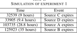
The application was simulated using the Castalia 1.3 simulator [17]. The nodes were based on the TMote sky [18]. The sink was given a near-infinite supply of energy and other nodes were given 14.58 J of energy. Experimental observations are shown in Table II.

Table II

SIMULATION OF EXPERIMENT1

Time Event

32539 (9 hours) Source C expires 33905 (9.4 hours) Source D expires 103735 (28.8 hours) Source A expires 125923 (35 hours) Source B expires

Source C was the first node to expire. However, its loss is unlikely to have rendered the network unusable since source D could be used in place of source C for routing. When source D expired, only sources A and B remained connected to the sink. However, it may have been possible to estimate the temperature gradient at future times using only A and B. If the network could remain usable with only sources A and B, then its useful network lifetime (35 hours) is almost four times greater than n-of-n lifetime suggests.

The network was then modified to that shown in Figure 2b by inserting an additional source J to the void between sources E and F in order to obtain a higher resolution temperature gradient. The observations are shown in Table III.

Table III

SIMULATION OF EXPERIMENT2

Time Event

28511 (8 hours) Source C expires 29450 (8.2 hours) Source D expires 105538 (29.3 hours) Source A expires 122628 (34 hours) Source B expires

ineffective at representing the usefulness of the network. Conversely, the CWT metric with x = 2 increased from

2.45×108 _to2.93×108 _{(19.6%). Thus, the CWT metric}

correctly reflected the improved temperature gradient that can be achieved by the introduction of source J whereas the data transfer metric incorrectly suggests that the addition of source J has a negative effect on the application.

VIII. CONCLUSIONS

We have argued that current WSN metrics are inappropri-ate for measuring applications that benefit from high source diversity. Classical approaches such as data transfer or sink connectivity do not compensate for the increased energy expenditure caused by sources routing data on behalf of other sources (the source forwarding problem) and may not be able to handle data aggregation. Connectivity Weighted Transfer is a new metric that is specifically designed to reward networks that maintain high source connectivity. By utilising a user defined weighting, an application’s perfor-mance can be measured according to its ability to keep numerous sources connected, as required by the user.

We are currently exploring a system based on node reliance, which we define as the extent to which a node is relied upon in (source, sink) routing. In particular, we are developing a family of routing protocols based on node reliance that maintain a high source diversity for as long as possible.

REFERENCES

[1] I. Dietrich and F. Dressler, “On the lifetime of wireless sensor networks,” ACM Transactions on Sensor Networks, vol. 5, no. 1, pp. 5:1 – 5:39, 2009.

[2] R. Szewczyk, A. Mainwaring, J. Polastre, J. Anderson, and D. Culler, “An analysis of a large scale habitat monitoring application,” in 2nd international conference on Embedded networked sensor systems. Baltimore, MD, USA: ACM, 2004, pp. 214–226.

[3] P. Zhang, C. M. Sadler, S. A. Lyon, and M. Martonosi, “Hardware design experiences in zebranet,” inConference on Embedded Networked Sensor Systems, Baltimore, MD, USA, 2004, pp. 227–238.

[4] N. Xu, S. Rangwala, K. K. Chintalapudi, and D. Ganesan, “A wireless sensor network for structural monitoring,” in Con-ference on Embedded Networked Sensor Systems, Baltimore, MD, USA, 2004, pp. 13–24.

[5] E. Miluzzo, N. D. Lane, K. Fodor, R. Peterson, H. Lu, M. Musolesi, S. B. Eisenman, X. Zheng, and A. T. Campbell, “Sensing meets mobile social networks: The design, imple-mentation and evaluation of the cenceme application,” in6th ACM Conference on Embedded Networked Sensor Systems, Raleigh, North Carolina, USA, 2008, pp. 337–350.

[6] G. Tolle, N. Turner, K. Tu, and P. Buonadonna, “A macro-scope in the redwoods,” in3rd International Conference on Embedded Networked Sensor Systems, San Diego, California, USA, 2005, pp. 51–63.

[7] Y. Kim, T. Schmid, Z. M. Charbiwala, J. Friedman, and M. B. Srivastava, “Nawms: Nonintrusive autonomous water monitoring system,” in 6th ACM Conference on Embedded Networked Sensor Systems, Raleigh, North Carolina, USA, 2008, pp. 309–322.

[8] J. Beutel, S. Gruber, A. Hasler, R. Lim, A. Meier, C. Plessl, I. Talzi, L. Thiele, C. Tschudin, M. Woehrle, and M. Yuecel, “Permadaq: A scientific instrument for precision sensing and data recovery in environmental extremes,” in The 8th ACM/IEEE International Conference on Information Process-ing in Sensor Networks, San Francisco, USA, 2009, pp. 265– 276.

[9] G. Werner-Allen, K. Lorincz, J. Johnson, L. Lees, and M. Welsh, “Fidelity and yield in a volcano monitoring sensor network,” in The 7th USENIX Symposium on Operating Systems Design and Implementation, Seattle, Washington, 2006, pp. 381–396.

[10] T. Arampatzis, J. Lygeros, and S. Manesis, “A survey of applications of wireless sensors and wireless sensor net-works,” in The 13th Mediterranean Conference on Control and Automation, Limassol, Cyprus, 2005, pp. 719–724.

[11] I. Khemapech, I. Duncan, and A. Miller, “A survey of wireless sensor networks technology,” inProceedings of the 6th Annual PostGraduate Symposium on the Convergence of Telecommunications, Networking and Broadcasting, Liv-erpool, UK, 2005.

[12] D. M. Blough and P. Santi, “Investigating upper bounds on network lifetime extension for cell-based energy conservation techniques in stationary ad hoc networks,” inThe 8th Inter-natonal Conference on Mobile Computing and Networking, Atlanta, Georgia, US, 2002, pp. 183–192.

[13] S. Baydere, Y. Safkan, and O. Durmaz, “Lifetime analysis of reliable wireless sensor networks,”IEICE Transactions on Communications, vol. E88-B, no. 6, pp. 2465–2472, 2005.

[14] A. Giridhar and P. R. Kumar, “Maximizing the functional life-time of sensor networks,” inFourth International Symposium on Information Processing in Sensor Networks, Los Angeles, California, USA, 2005, pp. 5–12.

[15] Y. Wu, S. Fahmy, and N. B. Shroff, “On the construction of a maximum-lifetime data gathering tree in sensor networks: Np-completeness and approximation algorithm,” in27th Annual Joint Conference of the IEEE Computer and Communications Societies, Phoenix, AZ, USA, 2008, pp. 356–360.

[16] B. Carbunar, A. Grama, and J. Vitek, “Redundancy and coverage detection in sensor networks,” ACM Transactions on Sensor Networks, vol. 2, no. 1, pp. 94–128, 2006.

[17] H. N. Pham, D. Pediaditakis, and A. Boulis, “From simulation to real deployments in wsn and back,” inIEEE International Symposium on a World of Wireless, Mobile and Multimedia Networks, Ieee, Ed. Espoo, Finland: IEEE Computer Society, 2007, pp. 1–6.

[18] Sentilla, “Tmote sky datasheet,”