Simulated Minimum Cramér Von Mises Distance Estimation for Some Actuarial and Financial Models

http://www.scirp.org/journal/ojs ISSN Online: 2161-7198

ISSN Print: 2161-718X

DOI: 10.4236/ojs.2017.75058 Oct. 25, 2017 815 Open Journal of Statistics

Simulated Minimum Cramér-Von Mises

Distance Estimation for Some Actuarial

and Financial Models

Andrew Luong

*

, Christopher Blier-Wong

École d’Actuariat, Université Laval, Québec, Canada

Abstract

Minimum Cramér-Von Mises distance estimation is extended to a simulated version. The simulated version consists of replacing the model distribution function with a sample distribution constructed using a simulated sample drawn from it. The method does not require an explicit form of the model density functions and can be applied to fitting many useful infinitely divisible distributions or mixture distributions without closed form density functions often encountered in actuarial science and finance. For these models likelih-ood estimation is difficult to implement and simulated Minimum Cramér- Von Mises (SMCVM) distance estimation can be used. Asymptotic properties of the SCVM estimators are established. The new method appears to be more robust and efficient than methods of moments (MM) for the models being considered which have more than two parameters. The method can be used as an alternative to simulated Hellinger distance (SMHD) estimation with a spe-cial feature: it can handle models with a discontinuity point at the origin with probability mass assigned to it such as in the case of the compound Poisson distribution where SMHD method might not be suitable. As the method is based on sample distributions instead of density estimates it is also easier to implement than SMHD method but it might not be as efficient as SMHD me-thods for continuous models.

Keywords

Compound Poisson Distribution, Double Exponential Jump Diffusion Distribution, Mixture Distribution, Robustness, Influence Functions

1. Introduction

In actuarial science or finance we often model losses or log-returns with

distri-How to cite this paper: Luong, A. and Blier-Wong, C. (2017) Simulated Minimum Cramér-Von Mises Distance Estimation for Some Actuarial and Financial Models. Open Journal of Statistics, 7, 815-833. https://doi.org/10.4236/ojs.2017.75058

Received: September 13, 2017 Accepted: October 22, 2017 Published: October 25, 2017

Copyright © 2017 by authors and Scientific Research Publishing Inc. This work is licensed under the Creative Commons Attribution International License (CC BY 4.0).

http://creativecommons.org/licenses/by/4.0/

DOI: 10.4236/ojs.2017.75058 816 Open Journal of Statistics

bution functions where neither the distribution function nor its corresponding density function has a closed form expression yet it is not complicated to draw random samples from these distributions. It is clear that likelihood methods are complicated in such a situation.

For statistical inferences using models with these features, we shall assume to have independent and identically distributed (iid) observations X1,,Xn

which have a common distribution as X with model distribution and density given respectively by F uθ

( )

and fθ

( )

u . Neither F uθ

( )

nor fθ

( )

u has a closed form expression but often its moment generating function (mgf) M_θ

( )

s

has a closed form expression. The vector of parameters of interest is

(

θ

1, ,

θ

m

)

′

= 

θ

The compound Poisson distribution used in actuarial sciences and jump dif-fusion distribution in finance are typical examples for these types of models. Furthermore, in many circumstances distributions derived from the increments of Lévy processes also display these characteristics and it is of interest to make inferences for the vector of parameters. We shall illustrate the situation with example 1 and example 2 below.

Example 1

In this example, we shall consider the compound Poisson gamma distribution which is commonly used in actuarial science and it arises from the compound Poisson processes which also belong to the class of Lévy processes.

The compound gamma distribution is the distribution of a random variable X representable as a random sum, i.e.,

1

N i i

X =

∑

₌Y with the Yi’s being iid with a common gamma distribution with

the density function given by

( )

( )

1 1

e , 0, 1, 0

y

Y

f y _α yα β y α β

α β

− −

= > > >

Γ and

the moment generating function is given by

( )

(

)

1

1

Y M s

sα

β =

− . The random

variable N follows a Poisson distribution with parameter λ>0 and it is

as-sumed that the Yi’s and N are independent.

Note that the moment generating function of X is

( )

( ( )1)

e MY s

Mθ s = λ − (1)

and from the mgf M_θ

( )

s the first there cumulants can be found and they are

given by

(

)

(

)(

)

2 3

1 , 2 1 , 3 1 2

c =

αβλ

c =

αβ λ

+

α

c =

αλ α

+

α

+

β

(2)

The vector of parameters is

θ

=

(

α β λ

, ,

)

′.

DOI: 10.4236/ojs.2017.75058 817 Open Journal of Statistics

Furthermore, continuous distributions created using a mixing mechanism also leads to continuous mixture distributions without closed form density but simu-lated samples often can be drawn from such distributions. These distributions are commonly used in actuarial science and they are given by Klugman et al. [1]

(pp. 62-65); see Luong [2] for other distributions with similar features used in actuarial science.

Lévy processes are also used in finance and they can be used as alternative models to the classical Brownian motion. The distributions of the increments of these processes can be more flexible than the normal distribution, they can be asymmetric and have fatter tail than the normal distribution. Consequently, they are more suitable to model log-returns of assets in finance. The following double exponential jump diffusion distribution is an illustration of an alternative dis-tribution to the normal disdis-tribution which is the disdis-tribution of the increments of a Brownian motion.

Example 2

The double exponential jump diffusion model is a special case of a larger class of jump diffusion models where the distribution for the jumps follows an asym-metric Laplace distribution instead of the classical normal distribution as in the classical jump-diffusion model introduced by Merton [3]. This distribution has six parameters and it has been studied by Kou [4], Kou and Wang [5]. A sub- model which is the double exponential jump diffusion model with only five pa-rameters has been found very useful for modeling log-returns of stocks, see Tsay

[1] (pp. 311-319). We shall call this model, the KWT model. Exact pricing for European call option for this model is also possible with the use of some special functions. The distribution can be represented as the distribution of X with

1

N i i X = +Z

∑

₌Y

The Yi’s are iid with a common distribution and mgf given respectively by

(

)

1

; , e , , , 0,

2 x

Y

f y x

ω η

ω η ω η

η

− −

= −∞ < < ∞ −∞ < < ∞ >

(3)

( )

2 2

e 1

s Y

M s

s

ω

η

=

− . (4)

The distribution function of the double exponential distribution is

( )

1 e 2

x

Y F y

ω η −

= _for x≤ω and

( )

1 1 1 e

2 2

x

Y

F y

ω η

− −   = + _ − _

  for

x>ω. (5)

Since this distribution has an explicit expression, simulated samples drawn from the double exponential distribution can be based on the inverse method.

Tsay [6] (p. 312) also gives additional properties of the distribution of Y, i.e., the mean and variance are given respectively by

( )

( )

2

, 2

E Y =ω V Y = η

(6)

Pois-DOI: 10.4236/ojs.2017.75058 818 Open Journal of Statistics

son distribution with parameter λ and Z has a normal distribution

(

2

)

,

N µ σ .

It is easy to see that the mgf of X is given by

( )

1 2 2 e_{2 2} 1 1 2

e e

s

s s _s

M s

ω λ

µ σ _η

θ

 

 −

+ _{ −} _

= _{. (7)}

From Mθ

( )

s , the first five cumulants can be found and they are given by

(

)

(

)

2 2 2 2 3

1 , 2 2 , 3 6

c = +µ λω c =σ +λ η +ω c =λ η ω ω+ (8) and

(

4 2 2 4

)

(

4 2 3 5

)

4 24 12 , 5 120 20 .

c =λ η + η ω +ω c =λ η ω+ η ω +ω (9)

The vector of parameters is

(

2

)

, , , ,

µ σ λ ω η

′

=

θ

.

For models introduced by these examples if we use methods of moments (MM) to estimate the parameters, the MM estimators will lack of robustness properties and they might not even be efficient as for models with more than two parame-ters, MM estimators will depend on polynomials of degree higher or equal to three hence will be unstable in the presence of outliers. Estimators based on em-pirical characteristic functions procedures such as the KL procedures of Feur-verger and McDunnough [7] involves an arbitrariness of choice of points to match the empirical characteristic function with its model counterpart which motivates us in this paper to extend Cramer-von Mises estimation to a simulated version (version S). The classical Minimum Cramer Von-Mises estimators (ver-sion D) are given by the vector _θˆ _{which minimize the objective function}

( )

(

( )

( )

)

2

1

1 n

n i n i i

Q F x F x

n =

=

∑

− _θ

θ _{or equivalently (10)}

( )

(

( )

( )

)

2

( )

d

n n n

Q

θ

=

∫

_−∞∞ F u −F u_θ F u (11)

as given by Duchesne et al. [8] with F un

( )

and F uθ

( )

are respectively the

sample and model distribution. The MCVM estimators are known to be robust,

( )

1

[

]

1 n

n i i

F u I x x

n =

=

∑

≤ is the commonly used sample distribution and I

[ ]

. is

the indicator function. Note that if it is easy to draw samples from F uθ

( )

, we can construct the simulated sample distribution function S

( )

F_θ u using S ob-servations drawn from F uθ

( )

similarly and minimize instead the following objective function

( )

(

( )

( )

)

2

1

1 n S

n i n i i

Q F x F x

n =

=

∑

− _θ

θ

₍₁₂₎

to obtain estimators. We shall call these estimators simulated MCVM (SMCVM) estimators and denoted them by the vector θˆS and we shall call this version,

simu-DOI: 10.4236/ojs.2017.75058 819 Open Journal of Statistics

lated methods such as methods based on indirect inference, see Garcia et al. [9], also see Smith [10]. Therefore, the method appears to be useful for actuarial science and finance where there are needs to analyze data using these types of distributions. It can also be viewed as a natural extension of the classical MCVM methods proposed by Hogg and Klugman [11] (p. 83) where the asymptotic properties of the estimators have been established by Duchesne at al. [8]. Like Simulated minimum Hellinger (SMHD) method proposed by Luong and Bilo-deau [12], the new method is robust and it is even easier to implement than SMHD method as it makes use of sample distribution functions instead of den-sity estimates. Furthermore, it can handle models like the compound Poisson model which displays a probability mass at the origin where SMHD method might not be suitable but comparing to SMHD estimators, the SCVM estimators might not be as efficient as the SMHD estimators for continuous models.

The paper is organized as follows. Following the approach in section 3 by Pakes and Pollard [13] (pp. 1037-1043) who make use of the Euclidean space and Euclidean norm to establish asymptotic properties of estimators, the Hilbert space 2

l is used in this paper with a natural norm extending respectively the

Euclidean space and the commonly used Euclidean norm. Asymptotic properties for both the CVM estimators and the SCVM estimators can be established using a unified approach by considering minimizing the norm of a random function to obtain estimators and they are given in section 2. This approach also facilitates the use of the available results of their Theorems given in section 3 by Pakes and Pollard [13] as most of the results of their Theorems continue to hold in 2

l . The

SMCVM estimators are shown to be consistent and have an asymptotic normal distribution. Their asymptotic covariance can be estimated using the influence function approach which were used by Duchesne et al. [8]. An estimate for the covariance matrix is also given in section 2 and by having such an estimate, it will make hypotheses testing for parameters easier to handle. Section 3 displays results of a limited simulation study using the compound Poisson gamma model and the double exponential jump distribution where we compare the SMCVM estimators with methods of moment (MM) estimators. For both models, it ap-pears that the SCVM estimators are much more efficient than MM estimators using the overall relative efficiency criterion.

2. Asymptotic Properties of the SCVM Estimators

2.1. The Space

l

2

and Its Norm

We can make use elegant results of Theorem 3.1 and 3.2 in section 3 of the paper by Pakes and Pollard [13] (pp. 1037-1043) to investigate asymptotic properties of CVM estimators and simulated CVM estimators (SCVM). For asymptotic re-sults of estimators using simulations in their seminal works, Pakes and Pollard

DOI: 10.4236/ojs.2017.75058 820 Open Journal of Statistics

more convenient to consider the Hilbert space 2

l with infinite dimension

which generalize the Euclidean space and the following norm . defined below which generalizes the Euclidean norm.

For an element l

(

xl,1,xl,2,

)

′ =

x  which belongs to l2, define

(

)

1

2 2 , 1 l i xl i

∞ =

=

∑

x assumed to be finite. Clearly, . is a norm for 2

l and it

generalizes naturally the Euclidean norm. Also, a vector

(

u1, ,up

)

′ =

u  is of

fi-nite dimension p, hence belongs to the Euclidean space then it belongs to 2

l

with

(

u1, ,up, 0, 0,

)

′ =

u   . The space l2 and the norm . have been

stu-died in functional analysis or real analysis, see Davidson and Donsig [14] (pp. 137-141) for example.

For a matrix A=

( )

a_ij ,i=1, 2,,j=1, 2, in l2, define

(

)

1

2 2 1 1 ij i j a

∞ ∞

= =

=

∑ ∑

A . With the space l2, most of the results of their Theorems

in section 3 are valid and only some minor changes are needed.

For estimation, we assume that we have a random sample which consist of n iid observations X1,,Xn from a continuous parametric family with

distribu-tion F u_θ

( )

. We also assumed that F_θ has no closed form expression but

si-mulated samples can be drawn from F u_θ

( )

.The commonly used sample

distri-bution function is denoted by F un

( )

. The vector of parameters is denoted by

(

θ

1, ,

θ

m

)

′

= _

θ

. Define the following vectors of random functions

( )

( )

1 ( )1

( )

( )

, , n n n , 0, 0,

n n

F x F x

F x F x

G

n n

′

 − − 

=  

  

θ θ

θ

(13) for version D and it is easy to see that

( )

2

(

( )

( )

)

2

1

1 n

n i n i i

G F x F x

n

θ =

∑

₌ − _{θ .}

₍₁₄₎

Equivalently,

( )

2

(

( )

( )

)

2

d

n n n

G

θ

=

∫

_−∞∞ F u −F u_θ F , (15)

if F u_θ

( )

has support on the real line and

( )

2

(

( )

( )

)

2

0 d

n n n

G θ =

∫

∞ F u −F uθ F , if F uθ

( )

is the distribution of a non-negative random variable. Using the set up given by section 3 in Pollard and Pakes [13], the classical MCVM estimators can be viewed as the vector of values

which minimize

( )

2

n

G

θ

or G_n

( )

θ as defined by expression (15). For the simulated version of MCVM estimation, i.e., version S, define

( )

( )

1

( )

1

( )

( )

, , , 0, 0,

S S

n n n

n n

F x F x F x F x

G

n n

′

 − − 

= _ _

  

θ θ

θ

(16)

with S

( )

Fθ u being the sample distribution function based on the simulated

DOI: 10.4236/ojs.2017.75058 821 Open Journal of Statistics

given by the vector θˆS is obtained by minimizing

( )

2

(

( )

( )

)

2

1

1 n S

n i n i i

G F x F x

n =

=

∑

− _θ

θ . (17)

Clearly, both versions of MCVM estimation can be treated in a unified way using this set up, we also have G

( )

θ < ∞ in probability. For both versions, let

( )

0

( )

1

( )

1 0

( )

( )

, , n n , 0, 0,

F x F x F x F x

G

n n

′

 − − 

= _ _

  

θ θ θ θ

θ

_,

( )

2

(

₀

( )

( )

)

2

( )

d _n

G θ =

∫

_−∞∞ Fθ u −F uθ F u and we have

( )

0

( )

p n

F u →Fθ u ,

( )

( )

( )

1

n p

G θ − G θ =o , with op

( )

1 being an expression which converges to 0 in probability.

We shall restate Theorem 3.1 given by Pakes and Pollard [13] (p. 1038) as-suming the space 2

l and its norm as defined earlier are used so that it is more

suitable for CVM estimation. The condition ii) which requires Gn

( )

θ0 =op

( )

1

in their Theorem 3.1 can be replaced by Gn

( )

θ0 =op

( )

1 as only this condition

is used in their proof. Note that the set up for their Theorem is very general, we only need to verify their conditions for estimators obtained by minimizing the objective function of the form

( )

( )

2

( )

or

n n n

Q

θ

= G

θ

G

θ

(18)

Theorem 1: Under the following conditions, the estimators given by the vec-tor θ _{converges in probability to} θ₀, the vector of the true parameters, i.e.,

0 p

→



θ θ .

1) Gn

( )

θ

 ≤op

( )

1 +infθ∈Ω Gn

( )

θ

, Ω is the parameter space assumed to be

compact.

2) Gn

( )

θ0 =op

( )

1 .

3) ₀

( )

1

( )

sup_{θ θ− >δ} G_n θ − =O_p 1 for each δ >0 , Op

( )

1 is an expression bounded in probability.

Clearly for the SMCVM estimators given by the vector θˆS which minimizes

( )

( )

2

n n

Q

θ

= G

θ

will satisfy condition 1) and 2) of Theorem 1 as

( )

2

0

p n

G

θ

→ only at θ θ= ₀ if the parametric family is well parameterized

which is the case in general. Note that the integrand of the integral defined by expression (10) is nonnegative and smaller or equal to one. Therefore, in proba-bility,

( )

0<Qn θ ≤1 for θ θ− 0 >δ δ, >0

The condition 3) is satisfied in general which implies consistency for the

SCVM estimators, we then have ˆ 0

p S_→

θ θ . Note that since Qn

( )

θ is always

parame-DOI: 10.4236/ojs.2017.75058 822 Open Journal of Statistics

tric models are only hybrid, i.e., with some discontinuity points such as in the case of the compound Poisson models. Now we turn our attention to the ques-tion of asymptotic normality for θˆS _{and discuss informally the arguments used}

to establish asymptotic normality for θˆS _{first and the formal arguments will}

follow subsequently from the proofs of Theorem 3.3 by Pakes and Pollard [13]

(pp. 1040-1043). A version of their Theorem 3.3 is restated as Theorem 2 below.

Since

( )

(

( )

)

2

n n

Q θ = G θ is not differentiable, the traditional Taylor expan-sion argument cannot be used to establish asymptotic normality of estimators obtained by minimizing

(

( )

)

2

n

G θ . Here, we assume G

( )

θ is differentiable

with derivative matrix Γ

( )

θ , it means Fréchet differentiable with respect to the norm . for 2

l ; see Luenberger [15] for the notion of Fréchet differentiability

and see chapter 3 of the book by Luenberger [15] for the notion of Hilbert space. If the property of differentiability holds then we can define the random func-tion a

( )

n

Q

θ

to approximate Qn

( )

θ with

( )

(

( )

)

( )

( )

0

( )(

0

)

2

0 ,

a

n n n n

Q θ = L θ L θ =G θ +Γ θ θ θ− (19)

Let θˆS _and θ* _{be the vectors which minimize}

( )

n

Q θ and a

( )

n

Q

θ

re-spectively. The ideas behind the proofs for asymptotic normality of Theorem (3.3) of Pakes and Pollard are if the approximation of the original objective function Qn

( )

θ which is not differentiable by a differentiable one namely

( )

a n

Q

θ

is of the right order then the vector θˆS _{which minimizes}

( )

n

Q θ and

*

θ , the vector which minimizes a

( )

n

Q

θ

are asymptotically equivalent, i.e., we

have:

1)

(

)

(

*

)

( )

0 0

ˆS ₁

p

n

θ

−

θ

= n

θ

−

θ

+o or using equality in distribution,

(

)

(

*

)

0 0

ˆS d

n

θ

−

θ

= n

θ

−

θ

and it is easy to see that θ* _{can be expressed}

explicitly as *

(

)

1

( )

( )

0 , 0

n G

− ′ ′

= − =

θ Γ Γ Γ θ Γ Γ θ since Ln

( )

θ is an affine

transformation.

2)

( )

_ˆS a

( ) ( )

* 1

n n p

Q

θ

=Q

θ

+o n− ,

( )

1

p

o n− is an expression converging to 0 in probability at a faster rate than 1

n− .

Note that the matrix Γ

( )

θ0 is of rank m with m columns but infinite

num-ber of rows given by

( )

0

( )

1

ij b n

= θ =

Γ Γ _with 0

( )

i _{, 1, , , 1, ,}

ij

j

F x

b i n j m

θ

∂

= − = =

∂  

θ

and

0,

1,

,

1,

,

ij

b

=

i

= +

n



j

=



m

An estimate of this matrix Γ Γ=

( )

θ0 is Γˆn and is defined by expression

(33) in section (2.2), consequently we can estimate 0

( )

i

j

F x

θ

∂ ∂

θ

by its estimate

_{, 1, , , 1, ,}

ij

b i n j m

− =  =  using the corresponding elements ˆ

( )

_,

n i j

Γ

ex-tracted from ˆ

n

DOI: 10.4236/ojs.2017.75058 823 Open Journal of Statistics

 _{Γ , ,}ˆ

( )

_{1, , , 1, ,}

ij n

b n i j i n j m

− = − =  = 

(20)

Under these conditions, it suffices to work with θ* _and a

( )

*

n

Q θ to derive

asymptotic distribution for of θˆS. A regularity condition for the approximation

is of the right order given by their Theorem 3.3 which is the most difficult to check is given as

( )

( )

( )

( )

( )

( )

0

0 1

2

0

sup 1

n

n n

p

n n

o

n

δ

− ≤ ₋

− −

= + +

G G G

G G

θ θ

θ θ θ

θ θ

by Pakes and Pollard [13] (p. 1040).

A slightly more stringent condition which obviously implies the above regu-larity condition is

( )

( )

( )

( )

0 0

sup 1

n n n n op

δ

− ≤ G −G −G =

θ θ

θ

θ

θ

. (21)

For simulated methods for this condition to hold, in general independent samples for each θ cannot be used, see Pakes and Pollard [13] (p. 1048). Oth-erwise, only consistency can be guaranteed for estimators using version S, see section 2.2.2 for the same seed issue. For version S, the simulated samples are assumed to have size U=τn and the same seed is used across different values of θ to draw samples of size U. These two assumptions are quite standard for simulated methods of inferences, see section 9.6 for method of simulated mo-ments (MSM) given by Davidson and McKinnon [16] (p. 384), also see Smith

[10] (p. S66) for this assumption for his simulated quasi-likelihood estimators. For numerical optimization to find the minimum of Qn

( )

θ , we rely on direct

search simplex methods which are derivative free. Chong and Zak [17] (pp. 273-278) provides a good overview of derivative free simplex algorithm.

2.2. Asymptotic Normality

In this section, we shall state Theorem 2 which is essentially Theorem (3.3) given by Pakes and Pollard [13] and comment on the conditions needed to verify asymptotic normality for the MCVM estimators for version D and S.

Theorem 2

Let θ be a vector of consistent estimators for θ0, the unique vector which

satisfies G

( )

θ0 =0.

Under the following conditions: 1) The parameter space Ω _{is compact.}

2)

( )

12 _inf

( )

n op n Gn

−

∈   ≤ _ _+

 

G θ _{θ Ω} θ

3) G

( )

. is differentiable at θ₀ with a derivative matrix Γ Γ=

( )

θ0 of full

rank

4) supθ θ−₀≤δ_n n Gn

( )

θ

−G

( )

θ

−Gn

( )

θ

0 =op

( )

1 for every sequence

{ }

δn of

positive numbers which converge to zero.

DOI: 10.4236/ojs.2017.75058 824 Open Journal of Statistics

6) θ0 is an interior point of the parameter space Ω, assumed to be compact.

Then, we have the following representation which will give the asymptotic distribution of θ _{in Corollary 1, i.e.,}

(

)

(

)

1

( )

( )

0 n 0 p 1

n

θ θ

− = − Γ Γ′ − nΓ′G

θ

+o , (22)

or equivalently, using equality in distribution,

(

)

( )

1

( )

0 0

d

n

n

θ θ

− = − Γ Γ′ − nΓ′G

θ

. (23)

The proofs of these results follow from the results used to prove Theorem 3.3 given by Pakes and Pollard [13]. For expression (22) or expression (23) to hold only condition 5) of Theorem 2 is needed and used in their proofs of Theorem 3.3 and there is no need to assume that nGn

( )

θ

0 has an asymptotic

distribu-tion. Clearly MCVM estimators or SCVM estimators are obtained by minimiz-ing Gn

( )

θ hence they will satisfy the condition 2) of Theorem 2 with

( )

n

G θ as defined by expression (14) or expression (17) depending it is

ver-sion D or verver-sion S being considered. Therefore, for version D,

(

)

( )

1

( )

0 0

d

n

n

θ θ

− = − Γ Γ′ − nΓ′G

θ

, G_n

( )

θ as defined by expression (13)

And for version S,

(

)

( )

1

( )

0 0

ˆS d

n

n

θ

−

θ

= − Γ Γ′ − nΓ′G

θ

, G_n

( )

θ as defined by expression (16).

From the result of the Theorem, it is easy to see that we can obtain the main result of the following corollary which gives the asymptotic covariance matrix of the estimators.

Corollary 1.

Let Yn= nΓ′Gn

( )

θ

0 , if n

(

0,

)

L

N

→

Y V and

( )

Γ Γ′ →p A, A is full

rank and symmetric then

(

0

)

(

0,

)

L N

n

θ θ

− → D with

( )

−1

( )

−1

=

D A V A

(24)

The matrices D and V depend on θ₀ , and we adopt the notations

( )

0 ,

( )

0

= =

D D θ V V θ .

These results are proved by Pakes and Pollard [13], see the proofs of their Theorem (3.3). We just need to verify these conditions are met for SMCVM es-timation. Before verifying these conditions for both versions of MCVM estima-tion, the following assumptions are needed to verify the condition 4 of Theorem 2 which is the most difficult condition to verify. We need to define the following sequence of functions,

{

gn

( )

θ

}

as it will be used later,

( )

( )

( )

( )

2

0 , 1, 2,

n n n

g θ =n G θ −G θ −G θ n= 

Assumption 1

1) As n→ ∞ and θ→θ₀, for version S of CVM estimation

( )

( )

(

)

(

( )

( )

)

{

0 0

}

{

(

0

( )

0

( )

)

}

2

| |

S S S

x x

E F_θ x −F_θ x F_θ x −F_θ x →E F_θ x −F_θ x , (25)

{}

|x .

DOI: 10.4236/ojs.2017.75058 825 Open Journal of Statistics

bracket.

2) The sequence of functions e

( )

n

g θ is differentiable with continuous partial

derivatives, e

( )

(

( )

)

n n

g θ =E g θ , the expectation is under θ0 and using the

usual conditioning argument, it can also be expressed

( )

{

(

( )

( )

)

}

{

(

( )

( )

)

}

( )

( )

(

)

(

( )

( )

)

{

}

)

( )

0 0

0 0 0

2 2

| |

|

2 d

e S S

n x x

S S

x

g nE F x F x nE F x F x

nE F x F x F x F x F_θ x

∞ −∞



=  − + −



− − −

∫

θ θ θ θ

θ θ θ θ

θ

(26)

For the condition 1) of Assumption 1 to hold we cannot use independent samples for different values of θ to draw simulated samples for version S of CVM estimation, otherwise

( )

( )

(

)

(

( )

( )

)

{

0 0

}

| 0

S S

x

E F_θ x −F_θ x F_θ x −F_θ x = and gen

( )

θ

cannot converge to

0 in probability. This justifies the same seed must be used to generate random samples for different values of θ.

We shall proceed to check the regularity conditions for both versions of MCVM estimation and note that Γ

( )

θ is the derivative of G

( )

θ in 2

l

means that Γ Γ=

( )

θ0 is the Fréchet derivative at θ θ= 0 with the property

( )

( )

0

(

0

)

(

0

)

n − n − − =o −

G θ G θ Γ θ θ θ θ

As for the Euclidean space, the sufficient condition for differentiability here only requires the partial derivatives

( )

j F_θ x

θ ∂

∂ being continuous with respect to

θ. For the notion of derivative in Hilbert space, see the notion of Fréchet deriv-ative in Luenberger [15] (pp. 171-177) which generalizes the notion of derivative of Euclidean space. The conditions (1-3) of Theorem 2 can be verified easily. The condition (4) of Theorem 2 will be met in general if Assumption 1 holds, see Appendix for details and justifications.

We proceed to find the asymptotic distribution for nΓ′Gn

( )

θ

0 . Using

ex-pression (22) and exex-pression (23), we shall obtain the asymptotic covariance matrix for the MCVM estimators for both versions. For version D, the asymp-totic covariance matrix has been obtained by Duchesne at al. [8] (p. 407), using the influence function approach with the statistical functional R F

( )

n being

de-fined as

( )

( )

(

( )

( )

)

0

( )

( )

0

( )

( )

0

0

0 d ,

n n n n

F u F u F u

R F G _−∞∞ F u F u F u

=

∂ ∂ ∂

′

= −Γ = − =

∂ ∂ ∂

∫

θ θ θ

θ

θ θ

θ

θ θ θ

and consider the vector of influence function

( )

( )

(

)

1

0

, _x

R F

IC x F F δ F

=

∂

= = + −

∂



 



 (27)

x

δ is the degenerate distribution at the point 𝑥𝑥, F=Fθ0, 0≤ ≤ 1.The

influ-ence function IC x1

( )

is bounded provided that

( )

0

F u

∂ ∂

θ

θ as a vector of

DOI: 10.4236/ojs.2017.75058 826 Open Journal of Statistics

is bounded which implies the MCVM estimators are robust for version D. We shall assume this property of bounded influence functions holds implicitly; we shall see this also makes version S robust. Furthermore, based on standard re-sults of robust estimation theory, the representations given by expressions (28) and (31) using influence functions are valid for the statistical functionals being considered. Now since R F

( )

θ0 =0,

( )

( )

0

(

( )

( )

0

)

1 1

( )

1

( )

1

1

n

n n n i p

nR F n G n R F R F IC x o

n =

′

= − Γ θ = − _θ =

∑

+ ₍₂₈₎

This is the influence function representation of R F

( )

n =Γ′Gn

( )

θ0 for

ver-sion D and we have

(

ˆ 0

)

(

0, 1

)

L

n

θ θ

− →N D with D₁=

( )

A −1V₁

( )

A −1 for

version D, V1 is the covariance matrix of IC1

( )

x , IC1

( )

x is given by

expres-sion (2.15) in Duchesne et al. [8] (p. 407), with

( )

(

( )

( )

)

0

( )

( )

0 0

1 x d

F u x = _−∞∞ δ u −F u ∂ F u

∂

∫

IC _θ θ _θ

θ (29)

( )

(

1

)

0

E IC x = , since

(

( )

)

( )

0 x 0

Eθ δ u =Fθ u .

Replacing ∂F0

( )

u

∂

θ

θ by

( )

ˆ

F u

∂ ∂

θ

θ and Fθ0

( )

u by F un

( )

in the above

ex-pression leads to approximate the vector

( )

1 x

IC by IC1

( )

x with its elements given by

( )



(

( )

)

ˆ

( )

1 1

1

, 1, ,

j n

l j j n j

l F x

IC x I x x F x l m

n = θ

∂

 

= _ ≥ _− =

∂

∑

θ 

An estimate for the covariance matrix V1 can be defined as 

(



( )

)

(



( )

)

1 1 1 1

1

.

n

i i

i x x

n =

′

=

∑

V IC IC

(30) Using V1, an estimate for the asymptotic covariance matrix of θˆ can be

constructed, see expression (2.15) and expression (2.13) given by Duchesne et al.

[8] (pp. 406-407). Clearly, the results for version D as given by Duchesne et al. [8] can be reobtained using this unified approach.

Note that the property of asymptotic normality continues to hold even the parametric model fails to be continuous and is only hybrid as in the compound Poisson gamma case. Using the arguments of the next paragraph to establish asymptotic normality, the same conclusion can be reached for version S. The de-rivation of the asymptotic covariance matrix D2 for the SCVM estimators is

similar. We shall make use of the notion of bivariate statistical functional intro-duced by expression (1.6) given by Reid [18] (pp. 80-81). This leads to define the bivariate statistical functional

(

, 0

)

S n B F F_θ ,

(

)

( )

(

( )

( )

)

0

( )

( )

0 0 0

, S S d

n n n n

F u B F F − ′ = _−∞∞ F u −F u ∂ F u

∂

= G

∫

θ

θ Γ θ θ _θ

DOI: 10.4236/ojs.2017.75058 827 Open Journal of Statistics

( )

(

)

2

0, 0

,

B F F

y τ

τ

τ _{= =}

∂ =

∂

IC 



, F_ is as defined by expression (27) and F_τ is

si-milarly defined with Fτ = +F τ δ

(

y−F

)

,

δ

y is the degenerate distribution at

y and 0≤ ≤τ 1. Note that IC1

( )

x as given by expression (29) can also be

reobtained using the bivariate statistical functional with

( )

(

)

1

0, 0

,

B F F

y τ τ = = ∂ = ∂ IC    .

Based on the expression defining

(

, 0

)

S n

B F F_θ , we have IC2

( )

y = −IC1

( )

y

and IC1

( )

x is identical for version D and S. Therefore, for version S, we have

the representation

(

)

( )

( )

( )

( )

0

0 1 1 1 2 1

,

1

S n

n U

n i i i i p

nB F F

n

n x y o

U

n = =

′

= − G =

∑

IC +

∑

IC +

θ

θ

Γ . (31)

Note that the size of the random sample drawn from the model distribution is U =τn and the y_i’s are iid and have the same distribution as the xi’s but the

i

y’s are independent of the xi’s as the simulated sample is independent from

the original sample represented by the data. Therefore,

( )

0

(

)

1

1

0, , 1

L n n N τ   ′ → = +_{ }  

G θ V V V

Γ _{. (32)}

It is also clear that the elements of Γ Γ′ _{are given by}

( )

( )

( )

0 0 _{d , 1, , , 1, ,}

ij n

i j

F u F u

a F u i m j m

θ θ ∞ −∞ ∂ ∂ = = = ∂ ∂

∫

θ θ   which converge in

probability to the corresponding elements

a

ij of the matrix A with

( )

( )

( )

0 0

0

d , 1, , , 1, ,

ij

i j

F u F u

a θ θ F u i n j m

θ θ ∞ −∞ ∂ ∂ = = = ∂ ∂

∫

θ   , i.e. (33)

( )

a_ij ,i 1, m j, 1, , .m

= =  =  A

2.3. An Estimate for the Covariance Matrix

for SCVM Estimators

The asymptotic covariance matrix of θˆS _{can be estimated if we can estimate}

( )

0

= θ

Γ Γ . Using a result given by Pakes and Pollard (p. 1043), an estimate for

Γ _{is the matrix}

(

ˆ 1

) ( )

ˆ

(

ˆ

) ( )

ˆ

ˆ _{, ,}

S S S S

n G n n G n G n m n G

n n n  _{+ − + −}    =     

G θ e G θ G θ e G θ

Γ     (34)

(

0, 0, ,1, 0, , 0

)

i= ′

e   with 1 occuring at the ith entry of the vector ei and

n n

δ −

=

 , 1

2

δ ≤ and in general we can let 1

2

δ = . Note that the columns of ˆ

n

Γ

DOI: 10.4236/ojs.2017.75058 828 Open Journal of Statistics

( )

0 i _{, 1, , , 1, ,}

j

F x

i n j m

θ

∂

= =

∂  

θ

as mentioned in section (2.2).

Therefore, using results of Corollary 1 we have the asymptotic for version S

(

ˆ 0

)

(

0, 2

)

L S

n

θ

−

θ

→N D with 2

( )

1 1

( )

1

1 1

τ

− −

 

= +_{ }

 

D A V A . (35)

The factor 1 1

τ

+ _{represents the loss of overall efficiency due to simulations}

and can be controlled if we let τ≥10. This factor is identical to the one for

si-mulated unweighted minimum chi-square method or the one for sisi-mulated qua-si-likelihood method, see Pakes and Pollard [13] (p. 1049), also see Smith [10] (p. S69). It suffices to estimate V1 then we can have an estimate for the asymptotic

covariance matrix of the SCVM estimators as clearly A can be estimated by

ˆ ˆ

n n

′ Γ Γ .

Define IC1

( )

x with its elements given by



( )

(

( )

)

( )



1 1

1

, 1, , ,

n

l j j n j jl

IC x I x x F x b l m

n =  

=

∑

_ ≥ _− − = 

 0

( )

j _{, 1, , , 1, ,}

jl

l

F x

b θ j n l m

θ

∂

= − = =

∂   are as given by expression (20).

An estimate for V1 for version S can then be defined as



(



( )

)

(



( )

)

1 1 1 1

1 n

i i

i x x

n =

′

=

∑

V IC IC . (36)

Consequently, an estimate D2 for D2 can be defined as



(

)

1

(

)

1

2 1

1 _{ˆ ˆ ˆ ˆ}

1 _τ n n n n

− −

 _{+  ′ ′}

 

 

=

D Γ Γ V Γ Γ

(37)

Clearly with D2 available, it will facilitate hypothesis testing for the

parame-ters of the model.

3. Numerical Study

3.1. MM Estimation for the Compound Poisson Gamma Model

The MM method consists of matching the empirical cumulants with its model counterpart to form estimating equations and solutions will give the moment es-timators. For the compound gamma model of example 1 this leads to the system of equations given by

(

)

(

)

3

(

)(

)

2 2 3

1 3 1

1

, 1 , n 1 2

n n i i

c X s c X X

n

λαβ λαβ α ₌ λαβ α α

= = = + =

∑

− = + + _.

The sample mean and variance are given respectively by X and s2, the

moment estimators can be obtained explicitly. Note from these equations let

(

)

3

3 2 2

n n

c r

s β α

= = + _{and 2n} 2

(

1

)

X s

r = =β α+ which implies 3

2

2 1

n n r r

α α

+ =

+ and

DOI: 10.4236/ojs.2017.75058 829 Open Journal of Statistics

for α with  2 3

3 2

2 n n

M

n n r r r r

α = −

− . Since the parameter α≥1, we might want to

de-fine the moment estimator as α_M =min

( )

α_M,1 . It is not difficult to obtain



2n ₁ M

M r

β

α

=

+ and M  

M M X

λ

α β

= _{the corresponding MM estimators for} β _and

λ and when we also consider the constraints imposed on β _and λ, this leads to define

_M min

(

_M, 0

)

β = β _and λ_M =min

( )

λ_M, 0 .

3.2. MM Estimation for the KWT Model

For the KWT model, there are five parameters so beside the first three empirical cumulants as defined above we also need the fourth and fifth empirical cumu-lants with

(

)

4 ₄

4 1

1

3 n

n i i

c X X s

n =

=

∑

− − ,

(

)

5 ₂

5 1 3

1

10 n

n i i n

c X X c s

n =

=

∑

− − and matching

1n 1, 2n 2, 3n 3, 4n 4, 5n 5

c =c c =c c =c c =c c =c will give the moment estimators as in

the previous example. It might be easier to let δ η₌ 2 _{and from these}

estimat-ing equations, it is not difficult to see that the followestimat-ing two equations 3 3

4 4

n n

c c

c =c

and 5 5

4 4

n n

c c

c =c depend only on δ and ω and can be solved numerically to

obtain the MM estimators for δ and ω which are given respectively by

δ

M

and ωˆ_M. Also, using the first three equations we obtain



 2  

(

2

)

 

3

2 1

3 , ˆ 2 ˆ , ˆ

ˆ 6 ˆ

n

M M n M M M M n M M

M M M c

c c

λ

σ

λ

δ

ω

µ

λ ω

ω

δ ω

= = − + = −

+ .

We might want to redefine these MM estimators by imposing  2

ˆ

0, 0

M M

λ ≥ σ ≥ . In the limited simulation study, we draw M =100 samples of size n=1000

for each sample and use U=10000,τ=10.

For the overall asymptotic relative efficiency (ARE) for the compound gamma model we use

( )

( )

( )

( )

( )

( )

ˆS _ˆS ˆS

MSE MSE MSE

ARE

MSE MSE MSE

λ α β

λ α β

+ +

=

+ +

 _  , the mean square errors (MSE) are

estimated using random samples and displayed in Table 1. The mean square er-ror of an estimator πˆ for π₀ is defined as

( )

(

)

2 0

ˆ ˆ

MSE π =E π π− .

The range of the parameters being considered is given by 2≤ ≤α 10,1≤ ≤λ 10,1≤ ≤β 10.

We find that the SCVM method is more efficient than MM method, the order of ARE gained by using SCVM method is illustrated with results displayed in

[image:16.595.207.541.103.207.2]

DOI: 10.4236/ojs.2017.75058 830 Open Journal of Statistics

Table 1. Compound Poisson gamma model with β=10 asymptotic overall relative effi-ciency between SCVM estimators and MM estimators.

α⋱λ 1.00 5.00 6.00 7.00 8.00 9.00 10.00

2.00 0.4726 0.0105 0.4970 0.6418 0.7768 0.0030 0.2702 4.00 1.1277 0.1560 0.0348 0.0929 0.0393 0.0000 0.2973 6.00 1.0468 0.0396 0.0906 0.0070 0.0449 0.0592 0.02834 8.00 0.9032 0.0196 0.0351 0.0124 0.0553 0.0068 0.0032 10.00 0.8560 0.0352 0.3730 0.0896 0.0010 0.0179 0.0180

The overall efficiency used for comparisons used is

( )

( )

ˆ

( )

_{( )}ˆ

( )

( )

ˆ .

S S S

MSE MSE MSE

ARE

MSE MSE MSE

λ α β

λ α β

+ +

=

+ +

 _ 

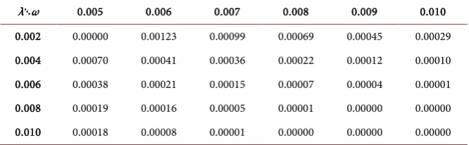
Table 2. Model KWT (µ=0.001,σ=0.001,η=0.02) asymptotic overall relative effi-ciency between SCVM estimators and MM estimators.

λ⋱ω 0.005 0.006 0.007 0.008 0.009 0.010

0.002 0.00000 0.00123 0.00099 0.00069 0.00045 0.00029 0.004 0.00070 0.00041 0.00036 0.00022 0.00012 0.00010 0.006 0.00038 0.00021 0.00015 0.00007 0.00004 0.00001 0.008 0.00019 0.00016 0.00005 0.00001 0.00000 0.00000 0.010 0.00018 0.00008 0.00001 0.00000 0.00000 0.00000

The overall efficiency used for comparisons used is

( )

( )

( )

( )

( )

( ) ( )

( )

( ) ( )

ˆ ˆ ˆ

ˆ ˆ

.

S S S S S

MSE MSE MSE MSE MSE

ARE

MSE MSE MSE MSE MSE

µ σ λ ω η

µ σ λ ω η

+ + + +

=

+ +  +  + 

 

similar findings.

For the KWT model we use the corresponding asymptotic relative efficiency (ARE) and it is defined as

( )

( )

( )

( )

( )

( )

( )

( )

( )

( )

ˆ _{ˆ ˆ}

ˆS ˆS S S S

MSE MSE MSE MSE MSE

ARE

MSE MSE MSE MSE MSE

µ σ λ ω η

µ σ λ ω η

+ + + +

=

+ +  +  + 

 

The mean square errors (MSE) are similarly defined as in the case of the compound gamma model and again estimated using simulated samples. The ARE is a ratio with the total of mean square errors for the SCVM estimators ap-pearing in the numerator and the total of mean square errors of MM estimators appearing in the denominator.

The key findings are illustrated using Table 2 and again SCVM method seems to perform much better than MM method for the common range of parameters used for modeling daily returns of stocks with

[image:16.595.207.540.281.384.2]

DOI: 10.4236/ojs.2017.75058 831 Open Journal of Statistics

resources to conduct larger scale of study being in a small department equipped with only laptop personal computers. Despite the limited nature of the study it does point to better efficiency when using SCVM methods for models having at least three parameters, in general.

4. Conclusion

It appears that SCVM method has the potential to generate more efficient esti-mators than MM method especially for models with more than two parameters. Like SMHD method, it is also robust and easier to implement than SMHD me-thod as it is based on sample distribution function instead of density estimates. It can handle continuous models with a few discontinuity points with probability masses attached to them where the SMHD method might not be suitable but it might be less efficient than SMHD method for continuous model, in general.

Acknowledgements

The helpful comments of an anonymous referee and the support of the staffs of OJS which lead to an improvement of the presentation of the paper are gratefully acknowledged.

References

[1] Klugman, S.A., Panjer, H.H. and Willmott, G.E. (2012) Loss Models: From Data to Decisions. New York, Wiley.

[2] Luong, A. (2016) Cramér-Von Mises Distance Estimation for Some Positive Infi-nitely Divisible Parametric Families with Actuarial Applications. Scandinavian Ac-tuarial Journal, 2016, 530-549. https://doi.org/10.1080/03461238.2014.977817

[3] Merton, R.C. (1976) Option Pricing When the Underlying Stock Returns Are Dis-continuous. Journal of Financial Economics, 3, 125-144.

https://doi.org/10.1016/0304-405X(76)90022-2

[4] Kou, S.G. (2002) A Jump Diffusion Model for Option Pricing. Management Science, 48, 1086-1101. https://doi.org/10.1287/mnsc.48.8.1086.166

[5] Kou, S.G. and Wang, H. (2004) Option Pricing under a Double Exponential Jump Diffusion Model. Management Science, 50, 1178-1192.

https://doi.org/10.1287/mnsc.1030.0163

[6] Tsay, R.S. (2016) The Analysis of Financial Time Series. 2rd Edition, Wiley, New York.

[7] Feuerverger, A. and McDunnough, P. (1981) On the Efficiency of Empirical Cha-racteristic Function Procedures. Journal of the Royal Statistical Society, Series B, 43, 20-27.

[8] Duchesne, T., Rioux, J. and Luong, A. (1997) Minimum Cramer-Von Mises Me-thods for Complete and Grouped Data. Communications in Statistics, Theory and Methods, 26, 401-420. https://doi.org/10.1080/03610929708831923

[9] Garcia, R., Reneault, E. and Veredas, D. (2004) Estimation of Stable Distribution by Indirect Inference. Journal of Econometrics, 161, 325-337.

https://doi.org/10.1016/j.jeconom.2010.12.007

DOI: 10.4236/ojs.2017.75058 832 Open Journal of Statistics Vector Autoregressions. Journal of Applied Econometrics, 8, S63-S84.

https://doi.org/10.1002/jae.3950080506

[11] Hogg, R.V. and Klugman, S.A. (1984) Loss Distributions. Wiley, New York. https://doi.org/10.1002/9780470316634

[12] Luong, A. and Bilodeau, C. (2017) Simulated Minimum Hellinger Distance for Some Continuous Financial and Actuarial Models. Open Journal of Statistics, 7, 743-759.https://doi.org/10.4236/ojs.2017.74052

[13] Pakes, A. and Pollard, D. (1989) Simulation Asymptotic of Optimization Estima-tors. Econometrica, 57, 1027-1057.https://doi.org/10.2307/1913622

[14] Davidson, K.R. and Donsig, A.P. (2009) Real Analysis and Applications: Theory and Practice. Springer, New York.

[15] Luenberger, D.G. (1968) Optimization by Vector Space Methods. Wiley, New York. [16] Davidson, R. and McKinnon, J.G. (2004) Econometric Theory and Methods.

Ox-ford.

[17] Chong, E.K.P. and Zak, S.H. (2013) An Introduction to Optimization. 4th Edition, Wiley, New York.

[18] Reid, N. (1981) Influence Functions for Censored Data. Annals of Statistics, 9, 78-92.https://doi.org/10.1214/aos/1176345334

[19] Rudin, W. (1976) Principles of Mathematical Analysis. McGraw-Hill, New York. [20] Newey, W.K. and McFadden, D. (1994) Large Sample Estimation and Hypothesis

DOI: 10.4236/ojs.2017.75058 833 Open Journal of Statistics

Appendix

In this technical appendix, we shall prove that with the conditions of Assump-tion 1, the condiAssump-tion 4 of Theorem 2 will hold, i.e.,

( )

( )

( )

( )

0 0

sup 1 ,

n n n n op

δ

= ≤ G −G −G =

θ θ

θ

θ

θ

i.e.,

( )

( )

( )

0 0

p

n n

n G θ −G θ −G θ → uniformly as θ→θ₀ and n→ ∞

Now define the sequence of functions

( )

( )

( )

( )

2

0

n n n

g

θ

=n G

θ

−G

θ

−G

θ

, it

suffices to show

( )

p 0

n

g

θ

→ uniformly as θ→θ0 and n→ ∞.

Using Markov’s type inequality, for any >0, we have the following

inequa-lity

( )

(

)

ne

( )

n

g P g ≥ ≤



θ

θ _with e

( )

(

( )

)

n n

g θ =E g θ as given by expression (26). Consequently, it suffices to have gne

( )

θ →0 uniformly as θ→θ0 and

n→ ∞. Clearly under Assumption 1 we have gne

( )

θ →0 pointwise but we need to strengthen it to uniform convergence for

{

e

( )

}

n

g θ . Therefore, it suffices to have equicontinuity for the sequence

{

e

( )

}

n

g θ as the domain of the sequence of functions is compact, see Rudin [19] (1974, p. 168). A sufficient condition for this property is the Lipschitz property which is related to the property of diffe-rentiability of the sequence of functions, see Davidson and Donsig [14] (2009, p. 88). Since the parameter space is compact and if the sequence

{

e

( )

}

n

g θ is dif-ferentiable hence Lipchitz then with Assumption 1, these properties implies equicontinuity for the sequences of functions

{

e

( )

}

n

g θ .