Actively Circulating Volume as a Consequence of
Stochasticity within Microcirculation
Viktor V. Kislukhin
Transonic Systems Inc., Ithaca, USA E-mail: victor.kislukhin@transonic.com
Received March 6, 2011; revised March 13, 2011; accepted March 16, 2011
Abstract
It is well established that in the pathology of the cardio-vascular system (CVS) only a portion of the blood volume (BV) can be in active circulation. This portion of BV is named the actively circulating volume (ACV) and is evaluated from a monotone decrease of dilution curve produced by an intravascular tracer. In given paper is presented Markov chain as a math model of the flow of a tracer throughout CVS. The consideration of CVS as a set of segments with respect to an anatomical structure and assuming the existence for CVS steady-state condition; leads to the Markov chain of the finite order with constant coefficients. The conclu-sions of the article are 1) there are open and closed microvessels, such that the switching from open to closed and back is a stochastic process, 2) if the switching is slow then the ACV, as the volume of heart chambers and only open for circulation vessels, can be detected.
Keywords:Blood Volume, Actively Circulating Volume, Microcirculation, Vasomotion, Markov Chain, Math Model of Cardiovascular System
1. Introduction
The importance of knowing BV is commonly accepted. However, BV is not routinely used in clinics or during experimental investigations. The primary drawback to measuring BV is that the mixing time for a tracer can vary from 2 - 3 min to 30 min [1]. Multiple blood-samp- ling method had been developed to solve the mixing di-lemma. However, as stated by Wiggers [2], if mixing of a tracer requires more then 10 min, the resulting volume is not the volume responsible for cardiac output and the distribution of blood pressure. Thus, the concept that only part of the BV is actively circulating was developed [2], meaning that the BV separates into ACV and slow circu- lating volume (SCV). The analysis of blood sample data is based on a two-compartment representation of BV, such that within the ACV a tracer mixes instantaneously, and a slow exchange occurs between ACV and SCV [3,4]. The calculation of ACV is based on the back extrapola-tion of the indicator’s concentraextrapola-tion decay to the time of injection [4,5]. ACV could be up to 50% of BV [5,6]. In this paper we address the question: what could be a cause for the monotone drop of the concentration toward a steady state concentration (this concentration is used for BV calculation [1]). To answer this question we exploit
the hypothesis made by Romanovsky in his monograph “Discrete Markov Chain” [6] that “the movement of blood particles in a human organism where the heart is the central point of branching, is a Markov (polycyclic) process.”
term corresponding to the complete mixing of a tracer; 2) the term of damped oscillations corresponding to the first pass and recirculation waves, and 3) the term of steadily (exponentially) decreasing items. An analysis of the con-ditions that enables the monotone decreasing term leads to the conclusion: the appearance of the SCV is due to the presence of closed microvessels and, additionally, the switching of the microvessels from the closed state to the open state and back is a slow process.
2. Mathematical Model for the Passage of an
Intravascular Tracer
We begin with the assumption: the future trajectory of any blood particle depends only on the current site of the particle. A model based on the given assumption is a Markov chain [10] if it includes the following three com- ponents: 1) a structure of the CVS, 2) a distribution of a tracer throughout the CVS, and 3) an operator of the transition of the tracer throughout the CVS. In detail:
1) A structure of the CVS. It is a set of segments {Sk; k
= 1 ··· N}, such as the heart chambers, conductive vessels and microvessels. The segments are enumerated. The numeration starts with the right atrium (RA) designated as S1. The numeration of other segments follows the rule
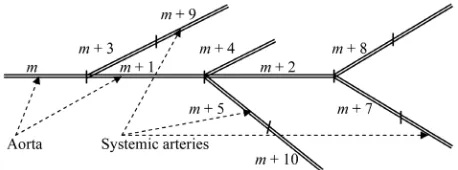
that blood flows from the segments with lower subscripts to segments with the higher subscripts. Only the segments connected with the RA are exceptions to this rule. Fig-ure 1 demonstrated the numeration of segments
begin-ning at the left ventricle.
2) Distribution of a tracer throughout the CVS. The distribution is a vector z(t) = {zk(t), k = 1, ···, N}, where
the kth component of z(t) is the fraction of a tracer within
the Sk at time t. As an initial distribution of a tracer, z(0),
will be taken z1(0) = 1, and for all k > 1 zk(0) = 0, mean-
ing that a tracer is injected into the right atrium at time t = 0,
3) Anoperator A = {aij} that provides the transition of
a tracer during one cardiac cycle, where the aij is the
fraction of a tracer within Si that passes during one car-
diac-cycle into Sj: As a result the distribution of the
trac-er at time t, z(t), transforms to the distribution at time t +
[image:2.595.58.287.609.694.2]1: z(t + 1) = z(t)A, and, recursively:
Figure 1. A possible numeration of the segments beginning with the left ventricle.
t
0 tz z A (1)
The text-book approach to dealing with (1) is to ex- pand it through the characteristic numbers, {si}, (the
roots of the equation Det(sA−E) = 0). Thus the dilution
curve recorded in the aorta, zm(t), is the power series of
three components:
1 1
1 cos
t t
m m mi i mj j j
z t b
b s
b s t (2) where, bm1, {bmi}, {bmj}, and {ωj} are the combinationsof eigenvectors of matrix A [10].
The examination of the components of (2) leads to the following:
1) The constant, bm1, corresponds to the concentration
of tracer after the mixing has been complited.
2) The second term, with all si real and > 1, is the
steadily decreasing term; it will be connected with the detection of ACV.
3) The damped oscillating term, with the frequencies of oscillations {ωj}. All sj are the complex numbers and,
by modulus, > 1.
3. Results
The main conclusion of this article is the consequence of the statement: if diagonal elements of A, are zero {aii = 0}
then the equation Det(sA – E) = 0 has only one real solu-
tion, s1 = 1. The proof follows from the statement that
two equations Det(sA – E) = 0 and F(s)=1 are equivalent
(see Appendix 1) (F(s) is the generating function of the first pass throughout CVS). The equation for F(s) is, see (A2):
k 1k
F s
p s (3) where pk is the fraction of a tracer that passes through theCVS (from RA to RA) in k-cardiac-cycles. Since the pk
add to 1, then s = 1 is the only real positive characteristic number. Taylor decomposition of (3) at s = 1, leads to the other characteristic numbers. They are
1 2 1 ; 1,
k
s ki F k .
with F
1 as the mean transit time (MTT) for passage throughout CVS. Conclusion: thus, zm(t), see (2), hasonly damped oscillations around bm1 and the frequencies
of damped oscillations are multiples of 2 F
1 . In other words, to have a steadily decreasing term in (2) we must have non-zero elements on the main diagonal of A. There are at least four aii > 0, and they correspond tothe heart chambers. However, the mean time to pass any heart chamber is about 2 - 3 cardio-cycles (in pathologi- cal enlargement of the heart the time to pass can be up to 20 cm3), thus the heart cannot be the cause of a monotone
must be non-heart elements aii > 0. The passage through
such segments can be described as follows: if in the i- segment a tracer stays for a while, we should have at least two segments, let them be numbered (i− 1) and (i + 1), such that the tracer enters i-segment from (i− 1) and lea- ves to (i + 1)-segment. Formally, from the (i − 1)-seg- ment a tracer partly enters the i-segment and could partly enter the (i + 1)-segment, these parts are ai − 1i and ai − 1i + 1,
and will be denoted as and = 1 −. A tracer from i- segment partly stays for the next cardiac-cycle, and partly passes to the (i + 1)-segment, these parts are aii and aii + 1,
and are denoted as and = 1 −. The generating func-tion to pass such construcfunc-tion is given by (4), see Appen- dix 2.
;1 s
v s s s
s
(4)
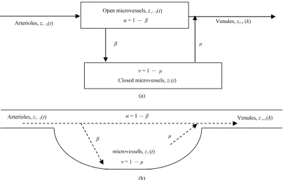
There are two realizations of the formal construction, see Figure 2:
1) Required segment (with aii > 0) contains microves-
sels closed for circulation, and (i− 1)-segment contains perfused microvessels. When closed microvessel beco- mes open its content passes to (i + 1) segment.
2) Segment (or a group of segments) is a mixing ch- amber, kind of “peripheral heart”.
The following reasoning is based on the first realize- tion. The first realization is chosen because 1) it is well established that practically in all tissues a part of micro- vessels is closed, and their recruitment is a way to res-
pond to an increase in flow [11,12]; 2) in muscle tissue it is established that a fraction of ink-containing capillaries depends on the time of infusion of ink. For 4 sec of the infusion the fraction of ink-containing capillaries is about 12%, and for 90 sec infusion there are 90% of ink-con- taining capillaries [13]; 3) despite the presence of a kind of “peripheral” hearts, they fall far from the needed rela-tion [volume]/[flow] be 3 - 9 min.
With non zero diagonal elements, the expression for a generating function for the passage of the CVS should include 1) the passage through the heart chambers with the generating function as 4
11
j j j
b s a s
, where aj and bjare residual and ejection fractions of j-heart chamber; 2) the passage through the systemic and pulmonary conduc- tive vessels; and 3) the passage through the microcircula- tion. The (5) gives the combined generating function, F(s), to pass throughout CVS, where F1(s) includes the
passage of the heart and conductive vessels, and the ex- pression in the brackets is the generating function of the passage through microcirculation, p1 + p2 = 1.
1
1 3
2 21 s F s F s p F s p F s s
s
(5)
Additionally to F(s), given by (5), we introduce the ge-nerating function, F0(s), to pass CVS if there is no
switching of the state (open/closed) of microvessels (= 0 and = 1, Figure 2):
(a)
[image:3.595.95.499.436.694.2](b)
Figure 2. Two possible realizations for non-zero elements from main diagonal of A. (a) Schematic for stochastic ex- change between open and closed microvessels; (b) Schematic for the passing of microvessels as a mixing chamber.
0 1 1 3 2 2
F s F s p F s p F s (6) Thus, our model of CVS has two distinct blood vol- umes:
1) Total blood volume, BV. By using established by Meier & Zierler [8] the relationship among mean transit time, flow, and volume we have:
1BV F SV, with SV as the stroke volume; (7) 2) A second blood volume, ACV, as the volume of open for circulation segments of CVS, such as heart chambers, conductive vessels, and open for flow micro-vessels. From (6):
1o
ACV F SV. (8) Now the aim of the article can be formulated as fol- lows: the volume given by (8) and the volume obtained by back extrapolation, if monotone decrease of zm(t) ex-
ists are the same. In Appendix 3, there are derivations of the next parameters:
1) The expression for a concentration after complete mixing occurs, bm11 F
1 .
1
1 1
m m
SV
z b
F BV
; (9)
2) The expression for the real characteristic number, s2 > 1,
2 1
BV s
ACV
(10)
with ACV as the volume given by (8)
3) The term bm2 1 F s
2 that is the factor at s2, andthe term 2 t 1
2 t mb s F s s is responsible for mono- tone decrease of zm(t). The back extrapolation of zm(t):
1 2
1 2
m m
m m
SV SV
b b ACV
ACV b b
(11)
By compare (8) and (11) one can conclude that ACV as the volume of the heart, conductive vessels, and open microcirculation and ACV obtained by the back extrapo- lation of zm(t) are the same.
From (10) one has the condition to have a clear mo- notone decrease of the concentration of the intravascular tracer toward the steady state (and consequently to have opportunity to measure ACV): the should be small, such as 1/ ~ 3 - 5 min (after cardiac cycles are transfor- med into minutes).
The volume SCV = BV – ACV with minutes consti- tuting the mean time of returning to the circulation could be used as the explanation for the disorder: 1) the bends from the removal of N2 since nitrogen in the tissue around
microvessels constituent SCV has slow removal; 2) the urea rebound, since removing of the urea in patients
un-der dialysis treatment from the tissue around of SCV is delayed [14]. Thus, the appearing of monotone decrease of zm(t) could be a the sign of microcirculation disorder.
There is a high probability that different parts of the microcirculation have different characteristics in the change of the state (open-closed) of microvessels. Con- sequently, (5) transforms into:
1
1 3
2 1
with 1
K
j j j j j
j j
i
s
F s F s p F s p F s s
s p
(12) This poses the main problem with the traditional me- thod for obtaining ACV. From Appendix 3 it follows that different in (12) lead to different real characteristic numbers, and the back extrapolation becomes dependent on the chosen time interval, the phenomena observed in the measurements of ACV [15].
4. Discussion
The main assumption, that leads to a Markov chain as a model for the transition of a trace throughout the CVS, is that every sequence of segments from the aorta to the right atrium and from the pulmonary trunk to the left atrium can be presented as a finite set. Two other assum- ptions are less significant. However, they simplify calcu- lations: 1) the stability of hemodynamic, meaning that matrix A is a constant matrix, and 2) the velocity of blood is the same throughout the cross-section of any vessel.
Since the work of Krogh it has been well established that the recruitment of microvessels is the leading res- ponse of the tissue to the demand for nutrients [11,16]. Experiments with ink infusion [13] have demonstrated that the longer the infusion time the more microvessels are exposed to infused particles. Thus, the indirect evi-dence for the involvement of closed microvessels into the circulation under the steady-state conditions is establi- shed.
5. Conclusion
ACV as the volume of heart chambers and only open for circulation vessels can be detected if the switching pro- cess is slow.
6. Competing Interests
The author declares that he has no competing interests.
7. References
[1] H. C. Lawson, “The Volume of Blood—A Critical Ex-amination of Methods for Its Measurement,” In: W. F. Hamilton and P. Dow, Ed., The Handbook of Physiology: Section 2, Circulation, Waerly Press, Baltimore, Vol. 1, 1962, pp. 23-49.
[2] C. J. Wiggers, “Physiology of Shock,” The Mechanisms of Peripheral Circulatory Failure, The Commonwealth Fund, New York, 1950, pp. 253-286.
[3] W. C. Shoemaker, “Measurement of Rapidly and Slowly Circulating Red Cell Volumes in Hemorrhagic Shock,” American Journal of Physiology, Vol. 202, No. 6, 1962, pp. 1179-1182.
[4] C. F. Rothe, R. H. Murray and T. D. Bennett, “Actively Circulating Blood Volume in Endotoxin Shock Measured by Indicator Dilution,” American Journal of Physiology, Vol. 236, No. 2, February 1979, pp. 291-300.
[5] A. Hoeft, B. Schorn, A. Weyland, M. Scholz, W. Buhre, E. Stepanek, S. J. Allen and H. Sonntag, “Bedside As-sessment of Intravascular Volume Status in Patients Un-dergoing Coronary Bypass Surgery,” Anesthesiology, Vol. 81, No. 1, July 1994, pp. 76-86.
doi:10.1097/00000542-199407000-00012
[6] V. I. Romanovsky, “Discrete Markov Chains,” Wolters- Noordhoff, Groningen, 1970.
[7] J. L. Stephenson, “Theory of the Measurement of Blood Flow by the Dilution of an Indicator,” Bulletin of Mathe- matical Biology, Vol. 10, No. 3, September 1948, pp.
117-121. doi:10.1007/BF02477486
[8] P. Meier and K. L. Zierler, “On the Theory of the Indica-tor-Dilution Method for Measurement of Blood Flow and Volume,” Journal of Applied Physiology, Vol. 6, No. 12, June 1954, pp. 731-744.
[9] R. Bellman, “Mathematical Methods in Medicine,” World Scientific, Singapore, 1983.
[10] W. Feller, “An Introduction to Probability Theory and Its Applications,” John Wiley & Sons Ltd., New York, Vol. 1, 1959.
[11] K. Zierler, “Indicator Dilution Methods for Measuring Blood Flow, Volume, and Other Properties of Biological Systems: A Brief History and Memoir,” Annals of Bio-medical Engineering, Vol. 28, No. 8, August 2000, pp. 836-848. doi:10.1114/1.1308496
[12] A. Krogh, “The Anatomy and Physiology of Capillaries,” Hafner Publishing Co., New York, 1959.
[13] E. M. Renkin, S. D. Gray and L. R. Dodd, “Filling of Microcirculation in Skeletal Muscles during Timed India Ink Perfusion,” American Journal of Physiology, August 1981, Vol. 241, No. 2, pp. 174-86.
[14] V. V. Kislukhin, “Vasomotion Model Explanation for Urea Rebound,” ASAIO Journal, Vol. 48, No. 3, May- June 2002, pp. 296-299.
doi:10.1097/00002480-200205000-00016
[15] T. Schroder, U. Rosler, I. Frerichs, G. Hahn, J. Ennker and G. Hellige, “Errors of the Backextrapolation Method in Determination of the Blood Volume,” Physics in Med-icine and Biology, Vol. 44, No. 1, January 1999, pp. 121- 301.doi:10.1088/0031-9155/44/1/010
[16] K. Parthasarathi and H. H. Lipowsky, “Capillary Re-cruitment in Response to Tissue Hypoxia and Its Depen-dence on red Blood Cell Deformability,” American Jour- nal of Physiology, Vol. 277, No. 6, December 1999, pp. 2145-2157.
Appendix 1
The expression for the determinant of the matrix B = sA
– E, if all main diagonal elements of A are zeroes.
To obtain the DetB let take b11= –1. By taking b11 we
are forced to take only the elements from the main di-agonal, thus the first term of DetB is (–1)N. To get other
terms of DetB let take the second non-zero element, sa12,
of the first row. The choice of next elements follows the repeatable procedure: 1) if the element saij is chosen, the
next element should be taken from j-row; 2) if in j-row there is the choice then the closest to the main diagonal element should be taken. The procedure continues unless we run into the element ak1. The product of all chosen
elements is 12 23 1
q k
a a a s . This is the fraction of a trace that passes CVS by the chosen path for the time in q-cardiac-cycles. The product becomes the term of DetB after multiplication by (–1)q + 1, and by all b
jj where j are
the numbers of the segments not presented in the given path. Since all bjj = −1, we have the term of DetB as:
1
12 23 1
1q q 1N q
k
a a a s
(A1) The (A1) establishes the one-to-one correspondence between the paths throughout CVS and nonzero elements of DetB, The sums of all terms of (A1) with the same
time to pass CVS, let it be q, is the fraction of injected tracer such that passes CVS in q cardiac-cycles. Let de-note this fraction as pq. With the use of {pq} the equation,
DetB = 0 can be written as:
1 1 M q q q p s
(A2) with the M as the longest path from RA to RA.. By the definition [10] the left part of (A2) is the generating function for the first time to pass through the CVS, and will be denoted as F(s).Appendix 2
The equations for the evolution of the part of the z(t) = (···, zi − 1(t), zi(t), zi + 1(t), ···), where subscript i denotes the
[image:6.595.55.541.515.741.2]non-heart segment of CVS with aii > 0, accordingly to
Figure 1 is:
1 1 1 1 1i i i
i i i
z t z t z t
z t z t z t
(A3)
Multiplying both parts of (A3) by st + 1 and summing
with respect to t, gives the following equation for con-nection between zi − 1(t), and zi + 1(t) in terms of a
gene-rating function:
1 1 1
1
t
i i i
t
s
Z s z t s s s Z s
s
(A4)where
1
s
v s s s
s
is the generating func-
tion for the passage through the segments (i – 1), (i), and (i + 1).
Appendix 3
The search for real characteristic numbers that are > 1.0. The equation v(s) = 1 has two solutions sv1 = 1 and
2 1 1
v
s . Between s1 and s2 there is the pole
1 1
p
s of v(s) and, consequently, of F(s). Since in the interval (sp, sv2) the F(s) varies from minus infinity
to F(sv2) > 1, F(s) = 1 has the solution in the given
inter-val. The use of Taylor decomposition of F1(s), F2(s), and
the difference for v(s) in the vicinity of sv2 (the difference,
not the derivative, is taken because of the proximity of the pole of v(s)) leads to the expression for the real cha-racteristic number >1:
1 1 3 2 2
2
1 1 3 2 2
1 1 1
1 1
1 1 1
F p F p F
BV s
F p F p F ACV
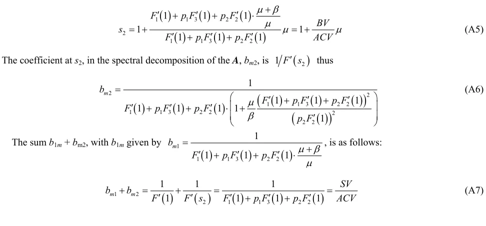
(A5)
The coefficient at s2, in the spectral decomposition of the A, bm2, is 1 F s
2 thus
2 2
1 1 3 2 2
1 1 3 2 2 2
2 2 1
1 1 1
1 1 1 1
1
m
b
F p F p F
F p F p F
p F (A6)
The sum b1m + bm2, with b1m given by
1
1 1 3 2 2
1
1 1 1
m b
F p F p F
, is as follows:
1 2
2 1 1 3 2 2
1 1 1
1 1 1 1
m m
SV
b b
F F s F p F p F ACV