Development and Application of Structural Equation Modeling Method For Geochemical Data Analysis

(1)

DEVELOPMENT AND APPLICATION OF

STRUCTURAL EQUATION MODELING METHOD

FOR GEOCHEMICAL DATA ANALYSIS

JIANGTAO LIU

A DISSERTATION SUBMITTED TO THE FACULTY OF GRADUATE STUDIES IN PARTIAL FULFILLMENT OF THE REQUIREMENTS

FOR THE DEGREE OF DOCTOR OF PHILOSOPHY

GRADUATE PROGRAM IN EARTH AND SPACE SCIENCE AND ENGINEERING YORK UNIVERSITY

TORONTO, ONTARIO October 2015 ©JIANGTAO LIU, 2015

(2)

ii

Abstract

A new Structural Equation Modeling (SEM) approach was proposed and the corresponding algorithms were designed and implemented for model estimation and evaluation in this research. By way of contrast to traditional SEM methods which focus on confirmatory analysis, the new SEM approach is mainly designed for exploratory analysis, which has plenty of applications in geoscience data processing and interpretation.

In order to generate an initial model for the new SEM analysis, a constrained variable clustering method was proposed based on a new index representing a type of conditional correlation, which was defined and calculated through SEM. Differently from the conventional conditional correlation coefficient, the new index was designed for measuring the quantity/percentage of the variance existing in two variables related to a response variable, rather than the level of independency of the two variables conditioned by a response variable. It can be used in Principal Component Analysis (PCA) and Factor Analysis (FA) for extracting factors restricted by a response variable. Thereby, these PCA and FA can be considered as constrained PCA and FA.

The programs designed for the new SEM are model parameters estimation, conditional correlation coefficient calculation, clustering analysis, and the SEM-based Weights of Evidence (WofE) modeling. The new SEM technology was applied to a lake sediment geochemical dataset to assist

(3)

iii

for identification of multiple geochemical factors related to gold mineralization in a study area located in Southern Nova Scotia, Canada. The model was further applied in conjunction with the WofE method to integrate geochemical and geological information in mapping mineral potential in the same study area. The results showed that the application of the new SEM method could reduce the effect of the conditional dependency of the evidences involved in WofE.

(4)

iv

Acknowledgements

I would like to express my special appreciation and thanks to my supervisors Dr. Qiuming Cheng and Dr. Jian-guo Wang, you have been a tremendous mentor for me. I would like to thank you for encouraging my research and for allowing me to grow as a research scientist. Your advice on both research as well as on my career have been priceless.

I would also like to thank Dr. Gunho Sohn, and Dr. Costas Armenakis for serving as my supervisor committee members. I want to thank you for your invaluable comments at each year’s research evaluation. I would extend my sincere thanks to the examining committees, Dr. Baoxin Hu, Dr. Eric Grunsky, Dr. Jarvis Gary, and Dr. Dong Liang, for letting my defense be an enjoyable moment, and for your brilliant comments and suggestions. I would like to take this opportunity to thank the Graduate Program Assistant and Administrative Assistant of ESSE at York University Mrs. Marcia Gaynor and Mrs. Paola Panaro, for your kindly help in the past six years. I would like to thank my friends in GIS research lab, Siping Xu, Xitao Xing, Wenlei Wang, Jie Zhao, Mangen Li，Gaifang Wang, Jingwei Gao, Deyi Xu, Quanming Liu, Yongzhi Wang and Guoxiong Cheng, for the happy time with all of your guys.

At the end I would like express special appreciation to my wife Huili Peng and my child Pengzheng Liu, without their trust in past years, this thesis would not have been possible.

(5)

v

Definition of Notation

x Independent measurement variable y Dependent measurement variable

Latent exogenous variable Latent endogenous variable

Modeling error associating the latent exogenous variables Modeling error associating the latent endogenous variables Modeling error associating the structural model

X Vector of independent measurement variables (x) Y Vector of dependent measurement variables (y)

Ξ Vector of latent exogenous variables ( )

Η Vector of latent endogenous variables ( )

Δ, Ε, Ζ Vectors of the modeling error terms ( , , ) Matrix

Β, Γ Coefficients (, ) in structural model

Μ Relationships ( ) between the observed variables and the latent variables Probability

P(A) Probability of event A

(6)

vi

P(A∪B) Probability that of events A or B

P(A | B) Probability of event A given event B occurred var(x) Variance of random variable x

σ2 Variance of a random variable

σx Standard deviation of random variable x

cov(x,y) Covariance of random variables x and y

Ry(xi,xj) A new conditional correlation between xi and xj under the restriction of y. ρx,y Correlation coefficient of variables x and y

. , Multiple correlation coefficient between y and { xi , xj } Px,y Direct effect of x to y

 Eigenvalue R2_(x

i,xj) The goodness of fit between xiand xj

Operators

∑ Summation - sum of all values in range of series ∑∑ Double summation

Others

SEM Structural equation modeling PLS-SEM Partial least square SEM

CB-SEM Covariance based SEM MLR Multiple linear regression

(7)

vii

Table of Used Geochemical Elements

Ag Silver As Arsenic Au Gold Cu Copper F Fluorine Li Lithium Nb Niobium Pb Lead Rb Rubidium Sb Antimony Sn Tin Th Thorium Ti Titanium W Tungsten Zn Zinc Zr Zirconium

(8)

viii

List of Tables

Table 1.1 Organization of multivariate methods ... 4

Table 3.1 Correlation coefficient between 16 elements in four formations ... 33

Table 3.2 Statistics of geochemical dataset ... 37

Table 4.1 Stages and steps in calculating the basic PLS-SEM algorithm ... 53

Table 4.2 The results obtained by the classification with As as the objective variable ... 60

Table 4.3 Regression coefficient from MLR and SEM. ... 64

Table 5.1 Estimated deposits number (T) under different combinations. ... 93

Table 5.2 Weights, contrasts and their standard deviations for predictor maps ... 106

Table 5.3 Weights, contrasts and their standard deviations for predictor maps …………..107

Table 5.4 The statistical result of posterio probability map in Fig 5.8A ... 110

Table 5.5 The statistical result of posterio probability map in Fig 5.8B ... 110

Table 6.1 Definition of parameters in Fig 6.1 ... 118

Table 6.2Correlation coefficient matrix ... 130

Table 6.3 Standardized new index Ry(x1,x2) under the restriction of As ... 131

Table 6.4 New index under the restriction of As ... 132

Table 6.5 Multiple correlation coefficient between {x1,x2} and As ... 133

Table 6.6 Correlation coefficient matrix for clr transformed data ... 152

Table 6.7 Standardized new index Ry(x1,x2) under the restriction of As for clr transformed data ... 153

(12)

xii

List of Figures

Fig 1.1 A chart showing recent SEM publication ... 8

Fig 1.2The calculation process in using traditional WofE for geo-data integration for mineral potential prediction ... 9

Fig 2.1 A flowchart showing a simple structural equation model consisting of one level of structure model and one level of measurement model ... 24

Fig 3.1 The study area in the Southern Nova Scotia, Canada. ... 31

Fig 3.2 Bed geologic units in the Southern Nova Scotia, Canada. ... 30

Fig 3.3 Locations of lake sediment samples in study area ... 34

Fig 3.4 Correlation coefficient between Au and other geo-chemical elements. ... 36

Fig 3.5 Correlation coefficient of As and Au in different rock units ... 36

Fig 3.6Histograms and boxplots for the concentration values of As ... 38

Fig 3.7 Histogram of 15 elements ... 39

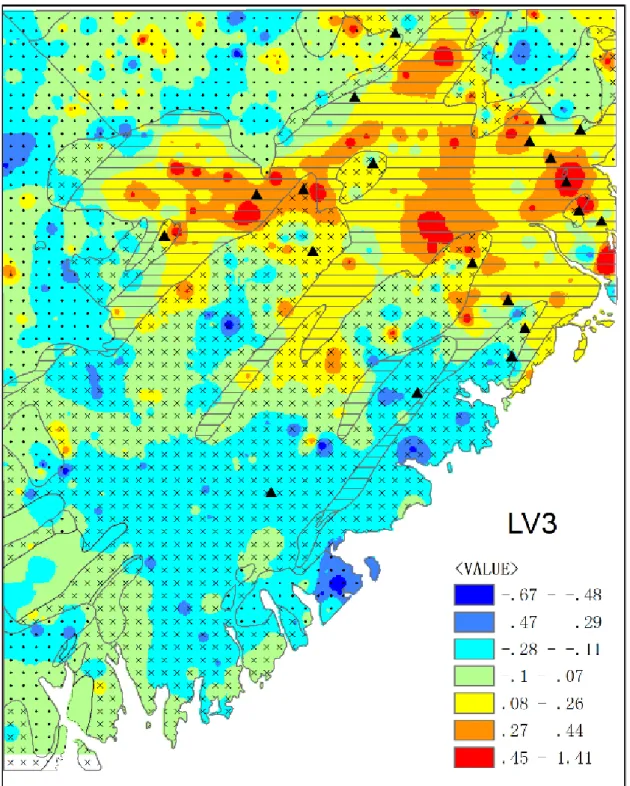
Fig 3.8 Spatial distribution of As, Au , Log10(As) and Log10(Au). ... 41

Fig 4.1Schematic chart showing an example of PLS-SEM. ... 50

Fig 4.2 A new method for estimating PLS-SEM parameters. ... 57

Fig 4.3 Regression coefficients of elements obtained by MVLR in each groups with Asas dependent variable... 62

Fig 4.4 A flowchart to show the structure of the SEM model for 15 elements as independent variables and As as depedent varaible ... 62

Fig 4.5 The regression coefficients in SEM (measurement model) and MLR. ... 65

(13)

xiii

Fig 4.7 Scores of 3 latent variables and factors obtained from SEM and FA, repectively.. .. 69

Fig 4.8 Scatter plots showing relationships between the calculated variables (latent variables and factors) and As ... 76

Fig 4.9 Maps showing the estimated values for As by three linear regression models(FA, SEM and MVLR).. ... 77

Fig 4.10 Scatter plots showing the observed value and predicted values of As.. ... 78

Fig 5.1 A re-classified layer for evidence.. ... 90

Fig 5.2 T-test values of evidences in Fig 5.1. ... 93

Fig 5.3 The relation between the number of estimated deposits and the combination index.93 Fig 5.4 The traditional WofE calculation process in geo-information integration for mineral exploration. ... 96

Fig 5.5 SEM of WofE method in mineral exploration.. ... 97

Fig 5.6 Evidences adopted in WofE calculation. ... 101

Fig 5.7 T-test values of four evidences. ... 105

Fig 5.8 The posterior probability map of deposits occurrence. ... 107

Fig 5.9 The regression between the predicted deposits and observed deposits. ... 111

Fig 5.10 The frequency of R square, over estimation ratio and target function value in sampling.. ... 112

Fig 5.11 The relationship between the over estimation ratio and R square. ... 113

Fig 6.1 A SEM between observed variables x and x and a response variable y ... 118

Fig 6.2 Relationships of Au with other elements in ρ _. _, , ρ _, , ρ _, , and R Au, x .. ... 125

Fig 6.3 Change in the relationships of Au with other elements in the standardized new index R Au, x and correlation coefficient ρ , ... 125

(14)

xiv

Fig 6.4 Relationships of Cu with other elements in ρ _. _, , ρ _, , ρ _, , and

R Cu, x .. ... 127 Fig 6.5 Change of relationships of Cu with other elements in the new index R Cu, x and

correlation coefficient ρ , ... 127

Fig 6.6 Relationships of Rb with other elements in ρ _. _, , ρ _, , ρ _, , and

R Rb, x . ... 129 Fig 6.7 Change of relationships of Rb with other elements in the standardized new index

R Rb, x and correlation coefficient ρ , . ... 129

Fig 6.8 Eigenvalues of the decomposition of three matrixes: correlation coefficient matrix,

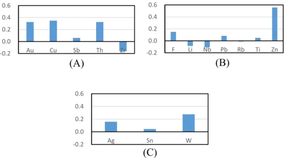
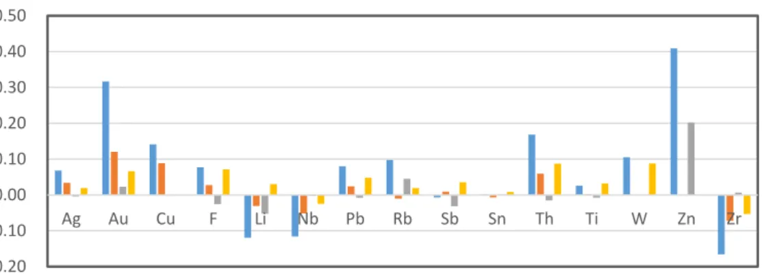
new index matrix and standardized new index matrix. ... 135 Fig 6.9 Loadings of components which calculated through the matrix of: correlation

coefficient, new index and standardized new index. ... 136 Fig 6.10 The absolute value of correlation coefficient of each component with As which

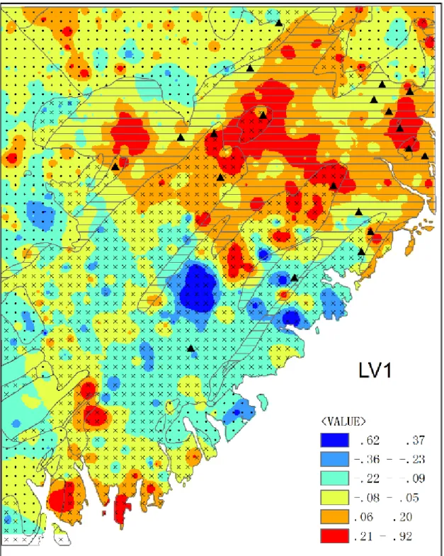
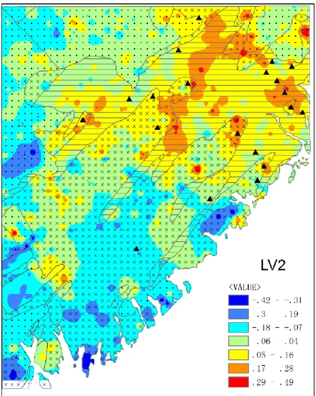
obtained through the matrix of correlation coefficient, new index and standardized new index ... 137 Fig 6.11 Score of calculated components through matrix of correlation coefficient, new index

and standardized new index. ... 138 Fig 6.12 Legend, north arrow and scale bar for Fig 6.11 ... 147 Fig 6.13 Hierarchical clustering (DINIA) results for 15 geochemical elements through

correlation coefficient matrix and standardized new index matrix.. ... 148 Fig 6.14 Hierarchical clustering (DIANA) results for 15 clr transformed elements through

correlation coefficient and standardized new index matrix... 154 Fig 7.1 Flow chart of the new clustering algorithm. ... 160 Fig 7.2 Hierarchical clustering results (CLV) for 15 geochemical elements based on

correlation coefficient matrix and standardized new index matrix.. ... 163 Fig 7.3 Centroid loadings in new index on elements in each cluster. ... 164

(15)

xv

Fig 7.4 The centroid of group 1, 2 and 3. ... 166 Fig 7.5 Prediction error through group 1, 2, 3 and all elements. ... 169 Fig 7.6 The first component of group 1, 2 and 3 calculated through the standardized new index

matrix. ... 175 Fig 7.7 The scatter map between the prediction of As and the first component based on

standardized new index matrix in group 1, 2, 3 ... 178 Fig 7.8 Hierarchical clustering results through CLV algorithm for 15 clr transformed elements

(16)

1

Chapter 1 Introduction

1.1 Statistics in geoscience

With the development of detection technology and the support of geographic information systems (GIS), the field of geo-data processing becomes more and more popular (Ali et al., 2007; Atekwana and Slater, 2009; Campo, 2012; Hart and Martinez, 2006; Jensen, 2009; Madden and Julian, 1994; Minasny et al., 2008; Mouillot et al., 2014; Nykiforuk and Flaman, 2009; Rao et al., 2008; Rollinson, 2014; Selva et al., 2014; Weng, 2014; Wielicki et al., 1996). In recent years, the volume of geo-data from multiple sources (e.g. real-time flood data, surface- and ground-water data; and information related to natural hazards, etc.) has increased rapidly. Also, the modern web technologies are making the utilization of geological and geospatial data increasingly global, accessible and instantaneous. Moreover, global energy and mineral crises, abnormal climate, and natural hazards etc. compel the geoscientists to provide more detailed and timely useful information from massive databases. Undoubtedly, it is a big challenge to extract and fuse information for useful applications in geoscience, which can be achieved using computer hardware (e.g. cloud technology), geoinformatics software (e.g., ArcGIS) and statistical methods. By considering the importance of extracting useful information from massive databases, the geo-data processing technology was listed as one of the future directions in solving the global challenges during 2007-2017 by the U.S. Geological Survey (GSurvey,

(17)

2

2007).

Mathematical methods have been playing a pivotal role in geo-data processing for several decades. Obviously, most of the techniques in quantitative geology are involving statistical approaches. Interest in areal or block averages for ore reserves in the mining industry led to the development of geo-statistical analyses in the 1950s, which aimed to provide quantitative descriptions of natural variables distributed in space and/or time. The development and proliferation of powerful personal computers have aided the widespread distribution of statistical software and sharable data over the internet through organizations such as the International Association for Mathematical Geosciences (IAMG). Some mathematical techniques have become standard practices in some geo-data processing. For example, the Principal Component Analysis (PCA) method can be used for extraction of geochemical factors (Cheng et al., 2011; Wang and Cheng, 2008), the Weight of Evidence (WofE) method can be used for mineral exploration (Agterberg, 1989; Agterberg and Bonham-Carter, 1990; Bandeen-roche et al., 1997; Bonham-Carter et al., 1988; Bonham-Carter et al., 1989; Bonham-Carter, 1994), and the Concentration Areal – Spectral Areal (C-A or S-A) methods have applied to detection of geological anomalies (Cheng et al., 2000; Cheng, 1999, 2007a, 2007b, 2012a, 2012b, 2014). The applied statistics is especially important in the petroleum and mineral industry, where it becomes instrumental in identification of anomalous mineralization and thus, provides more precise target areas for exploration.

(18)

3

practitioners, and the governmental agencies. Although high volume of geological data is now readily available, there is a dearth of professionals utilizing their analytical skills to understand and extract useful information from the data. Geo-data analysis requires rigorous scientific approaches, which rely on knowledge of statistics, measurements, logic, theory, experience, and situational context (Harris et al., 2015; Gao et al., 2014; de Caritat and Grunsky, 2013;

Grunsky et al., 2014; Savinykh and Tsvetkov, 2014; Wathne et al., 1996). Therefore, it is crucial to extract useful, accurate and timely information from geo-data sets that use multiple sources (e.g. GIS and Remote Sensing) and levels (e.g. multi-level resolution and completeness data). For example, the WofE method is one of the most popular methods for information fusion in mineral exploration (Agterberg, 1989; Agterberg and Bonham-Carter, 1990; Agterberg and Cheng, 2002; Bonham-Carter et al., 1988; Cheng and Agterberg, 1999). With this method, an evidence is considered as a dependent variable when being extracted from a multi-source data (e.g. geochemical element variables, geophysics variables, and geologic features). It is considered as an independent variable in calculating of the posterior probability of mineralization. Because the evidences are estimated without considering the conditional independence (CI), it makes them hard to meet the CI requirement when they are adopted in the calculation of the posterior probability. In order to solve this problem, there are several methods that have been proposed for testing the CI (Bonham-Carter et al, 1989; Agterberg,

1992; Bonham-Carter, 1994; Agterberg and Cheng, 2002) and reducing the effect of it in mineral prediction (Bonham-Carter,1994; Journel, 2002; Krishnan et al. 2004; Polyakova and Journel, 2007; Cheng, 2008, 2015; Deng, 2009, 2010a, b; Zhang et al., 2009; Agterberg, 2011; Schaeben, 2012).

(19)

4

Structural Equation Modeling (SEM) can be defined as a class of methodologies that seeks to represent hypotheses about the means, variances, and covariances of observed data in terms of a smaller number of ‘structural’ parameters defined by a hypothesized underlying conceptual or theoretical model (Kaplan, 2008). It provides a statistical approach to testing hypotheses about relations among observed and latent variables (Hoyle, 1995), which has been widely applied in social and behavioral sciences. This method may be applied to address the multi-level, and multi-model problems in geo-data processing. The definition of SEM was articulated by geneticist Sewall Wright (1921), economist Trygve Haavelmo (1943) and cognitive scientist Herbert A. Simon ( 1977), and formally defined by Judea Pearl ( 2000) using a calculus of counterfactuals. As shown in Table 1.1, SEM is considered as a second generation statistical

technology (Fornell, 1987; Lohmöller, 1989; Hair Jr et al., 2013).

Table 1.1 Organization of multivariate methods (Hair Jr et al., 2013)

Primarily Exploratory Primarily Confirmatory 1st_generation _{Cluster analysis}

Exploratory factor analysis Multidimensional scaling

Analysis of Variance Logistic regression Multiple regression 2nd_generation _PLS-SEM _{CB-SEM, including}

Confirmatory factor analysis In recent years, proliferation of computer hardware and software along with more user-friendly interfaces has enabled SEM to become more and more popular. Its theory and statistical properties have well been developed and found plenty of applications across many disciplines including education, psychology, sociology, and environmental epidemiology (Browne and

(20)

5

Arminger, 1995; Muthen, 1984; Sánchez et al., 2005; Yuan and Bentler, 2000; Yuan and Bentler, 1997). In mainstream statistical journals, SEM theory has also appeared under the terms “mean and covariance structures” and “latent variable models” (Bandeen-roche et al., 1997; Jöreskog, 1970, 1978; Lee and Shi, 2001; Sammel and Ryan, 1996; Yuan and Bentler, 1997). The advantages of SEM over first generation statistical technologies can be characterized as follows (Hair Jr et al., 2013):

1. SEM allows making use of several indicator variables per construct simultaneously, which leads to more valid conclusions on the construct level. Using other methods of analysis would often result in less clear conclusions, and/or would require several separate analyses.

2. SEM allows modeling and testing complex patterns of relationships, including a multitude of hypotheses simultaneously as a whole (including mean structures and group comparisons).

3. SEM provides a confirmatory approach for complex models. For hypothesis, simple statistical procedures usually provide tests on the basis of explained variance in single criterion variables. This may not be suitable for evaluating complex models containing a multitude of variables and relationships. In contrast, SEM allows to test complex models for their compatibility with the data in their entirety, and allows to test specific assumptions about parameters for their compatibility with the data. This allows for global assessment, local assessment and exploratory suggestions for potential model improvements (modification indices).

(21)

6

Geochemical data is typically reported as compositions, in the form of some proportions such as weight percents, parts per million, etc., subject to a constant sum (e.g. 100%, 1,000,000 ppm). The relations of elements in components are different with which in real sample space, i.e. in correlation analysis, the compositional data may result a type of spurious correlations among components if they are processed as unconstrained vector, which was pointed out by Karl Pearson in his 1897 paper (Pearson, 1896) firstly. For overcoming the problems of compositional data in geo-data processing, Aitchison (1982, 1984) introduced proper representations of a composition in order to have all the relevant information contained in a set of log-ratios. The additive log-ratio (ALR) (Aitchison, 1986) is one of the methods proposed for compositional data transformation, in which one part of compositions is chosen as the common denominator of all the ratios. In order to overcome the inconvenience of ALR which depends on the permutation of the components, Aitchison (1986) introduced a centered log-ratio transformation (CLR) to represent a D-part composition using D CLR-coefficients. The CLR transform does not result in an orthonormal space. Thus standard parametric modelling procedures cannot be applied. Egozcue et al. (2003) proposed the isometric log-ratio transformation (ILR) to work with orthonormal bases and their corresponding coordinates. More information about compositional data analysis can be found in recent publications

(22)

7

1.2 Motivation

The motivation to explore the use of SEM in geo-data processing mainly comes from the followings:

1) A structural equation model, as a combination of a measurement model to define latent variables using one or more observed variables, and a structural regression model to link latent variables together, is found on several multivariate statistical analysis methods, e.g. Factor analysis, PCA, Multi-linear regression, Path analysis, Latent variable analysis, which are very popular in geoscience data processing.

SEM is a combination of many multivariate statistical models, each of which can be considered as a special case of SEM. For example, in SEM, while the measurement model is analogous to factor analysis, the structural model may be considered analogous to multi-linear regression. Since both the factor analysis and multiple linear regression methods are widely used in the geo-data analysis, the SEM method may be more suitable for cases where the former methods can be applied.

Also, SEM is a popular concept in many disciplines. As a fact, since the year of 2000, hundreds of papers relating to SEM have been published. The statistics showed that there were relative fewer papers related to SEM in the geosciences (Fig 1.1) from 2000 to 2009 (McArdle and

Kadlec, 2013), although it has widely been applied in social sciences, arts and humanities. It should be noted that SEM is a class of methodologies, part of this concept has been discussed

(23)

8

and applied in geo-data analysis (Harris et al., 2015), but the SEM discussed in current research is a narrowly defined method which include at least one measurement model and one structural model. For applying SEM in geoscience data analysis, one of the main difficulties is that a predefined model is required in SEM calculation, but it is usually hard to precisely define before analysis.

Fig 1.1 A Chart of SEM publications from 2000 - 2009.(McArdle and Kadlec, 2013)

2) In order to handle multi-level and multi-process problems to address the challenges in geo-data processing, SEM might be potentially adoptable due to its capability of combining concept and process.

The major challenge of combining concept with process is not only about creating a model to express the idea but also estimating a set of parameters to match the designed model. Taking the method of ordinary weights of evidence (WofE) as an example, the conventional WofE

0 20 40 60 80 100 120 2000 2001 2002 2003 2004 2005 2006 2007 2008 2009

Biology, Life Sciences, and Environmental Science Business, Administration, Finance, and Economics Chemistry and Materials Science

Engineering, Computer Science, and Mathematics Medicine, Pharmacology, and Veterinary Science

Physics, Astronomy, and Planetary Science Social Sciences, Arts, and Humanities

(24)

9

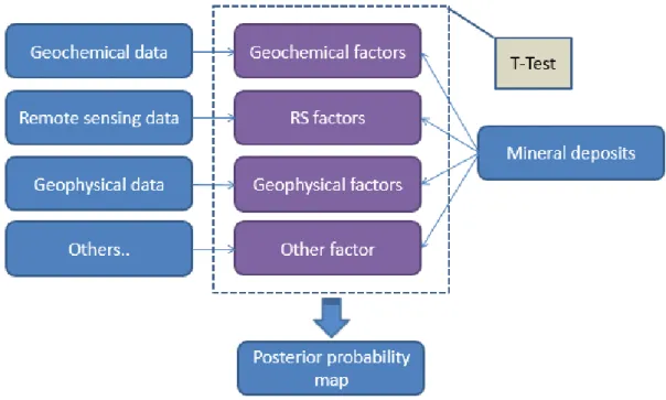
integrates multiple evidence layers that are of conditional independence from each other with respect of a point event. An evidence can be considered as a latent variable that cannot be measured/observed directly but extracted from raw data. The process of constructing evidences is analogous to factor analysis. However, it is considered as an independent variable when used in WofE for estimating the posterior probability of point event. This process is analogous to logistic regression. The traditional WofE has been implemented through two separate modeling

processes (Fig 1.2): extracting the evidences from

geochemical, remote sensing, and geophysical data; and then combining the evidences by a

Fig 1.2The traditional WofE calculation process in geo-data integration for mineral prediction

(25)

10

main information in source data, the extracted evidences are hard to meet the CI assumption of WofE method.There are several ways developed in the literature for solving the problem. In the current work it explores alterative solution to partially solve the problem by creating an SEM model to combine the factor analysis and regression, and further estimate the parameters with a global optimum function.

3) Application of SEM in geoscience is an interdisciplinary approach and has great potential for future research in the field.

As two popular methods in geo-data processing, PCA and FA can be considered as two special cases of SEM, which are processes to extract several “latent variables” through a measurement model. At the same time, SEM has been extended many subjects already, For example, similar as random forest and artificial neural network, SEM tree can be used for a decision (Oztekin et al., 2011; Brandmaier et al., 2013), which provides a data-driven but theory-constraint search in model space. Similar as the Dempster-Shafer, some of the SEM’s extension can be used for information integration too (Punniyamoorthy et al., 2011; Steinberg, 2009), i.e. the proposed SEM based WofE method in current research.

The broad successful SEM applications in social science indicate that SEM is not only about establishing a mathematic model in data processing, but also about developing a software tool, which includes to design the model in graphics, output calculation results in tables and graphics and manage projects. For the same reason, the application of SEM in geosciences will depend on both of the correct, efficient mathematic model and the software which is in line with the

(26)

11

practice of geoscientist. This demands for a good understanding in statistics, geoscience and computer science as well, which definitely increases the challenge of this research, but on the other hand, it provides moreavenue for innovation because its interdisciplinary nature.

1.3 Objectives

The overall goal of current research is to expand the application of SEM into geo-data processing and analysis. Based on a systematic study of the SEM concept, model, software and application, the feasibility of this method in geo-data processing will be tested and an efficient software tool for geoscience research will be provided.

The research of this proposal includes the following THREE objectives:

1) Apply SEM in geo-data processing and analysis to address the problems in multi-level models with latent variables, i.e. the implementation of WofE in mineral exploration. The successful application of SEM in mineral prediction may provide not only a new tool for geo-data processing, but also a new concept for information extraction and integration. The core idea in the SEM approach is to use a global optimum target function instead of gradually optimal methods to estimate a geological model involving multiple levels and processes.

2) Compose and develop a new SEM for geo-data analysis and accordingly design the algorithm and program for implementation: The second objective of this research is to propose the modeling methods and algorithms using C# and R programming languages, which includes

(27)

12

algorithm design (regression, factor analysis, and clustering), GIS function and user interface, etc. The proposed SEM method is designed as a software package in R, which allows efficient analysis of geo-data.

3) Validate the new method and software through case studies. The newly designed method and the developed software tools will be validated through a geochemical dataset obtained from 671 lake sediment samples. This process would include the identification of geochemical factors in regression to gold mineralization endogenous variables, and the integration of geochemical factors and geological factors for mineral potential mapping in the southwestern Nova Scotia, Canada.

In order to achieve the objectives, the following tasks have been conducted:

1) Exploration of the challenges of SEM in geoscience applications: Although SEM has many advantages over the traditional statistical techniques and great potential in a broad range of the applied scientific research, its application in geological data processing comes with some statistical and interpretational challenges, primarily due to the inherent nature of geoscience data (e.g., the problem in model identification / parameter estimation based on fuzzy model). A multitude of parameters (path coefficients, factor loadings, variances, etc.) corresponding to various hypotheses are estimated simultaneously so that the empirical relationships between the observed variables can be reproduced by the model in a robust manner. This is possible when the empirical data can provide adequate and correct information to estimate all these parameters. However, in most cases, geoscience data is a combination of "cascading" and/or "nesting",

(28)

13

further complicated by "masking" and "swamping" of under sampled processes. Therefore, part of this research will be to devise a method to extract an optimal geological process/model from a series of candidate processes/models using SEM.

2) Generation of an initial model: An initial model is required for a SEM application both for exploratory and confirmatory analysis. It may not be a big problem for some confirmatory analysis if the target of the research is to test some hypothesis, where the researchers usually have a model beforehand and then collect data related to their model, which is usually tested by some parameters such as the goodness-of-fit. But for some analysis in geoscience (e.g., mineral prediction, oil pipe route designation, urban planning, etc.), the relationships between different variables in a preliminary model is not clear prior to the analysis. For example, in mineral exploration, there exists some knowledge of the relationships between the ore-mineralization controlling factors. However, the detailed relationships among most of the factors are not obvious. Therefore, “generating the initial model” becomes the first problem which needs to be solved in order to apply SEM for geo-data processing.

3) Evaluation of the new model parameters: There have been two types of SEM: Covariance-based SEM (CB-SEM) and Partial Least Squares-Covariance-based SEM (PLS-SEM) developed for different applications (Hair Jr et al., 2013). CB-SEM is usually applied to model testing or confirmatory analysis. In mineral exploration, this means creating a model based on previous studies, conclusions and testing whether the model hypothesis is true. Hoyle and Panter (1995)

recommended some indexes about overall model fit (e.g. unadjusted chi-square) for hypothesis testing. The PLS-SEM method is mostly applied in the exploration analysis using an undecided model, where a regression of mineral-related targets can be specified to extract some latent

(29)

14

variables, which may subsequently be used in mapping the probability of mineral occurrence. The challenges faced in model estimation and evaluation chiefly come from the special nature of geo-data. For example, the geochemical data are influenced by combination of multiple sources and geological processes. Therefore, the variance and covariance of the data was decided by the source/ process providing the largest information, which maybe not the one we are interested in. However, in the CB-SEM method, the evaluation of the SEM model is based on Chi-square and some fitting indexes, all of which are calculated from the variance/covariance matrix. This method directly affects the final calculation if the variance/covariance does not represent the required information. A modified PLS-SEM as proposed in this research, may remove redundant information and extract respondent latent variables for a specified target.

4) Application of SEM concept into WofE for mineral prediction: The weight of evidence (WofE) is an artificial intelligent quantitative method based on the application of Bayes’ rule. The method, originally designed for a non-spatial application in medical diagnosis (Agterberg, 1989), is one of the most popular models using Bayes’ theory of conditional probability to quantify spatial association between evidence layers (or geological factors) and known mineral occurrences (Agterberg, 1989; Bonham-Carter, 1994; Carranza, 2004; Cassard et al., 2008; Porwal et al., 2010). Besides, WofE is applied to map landslide sensitivity evaluation (e.g., Lee and Choi, 2004; Neuhäuser and Terhorst, 2007; Regmi et al., 2010; Cervi el al., 2010), and ecology mapping (e.g., Calcerrada and Luque, 2006; Cho et al., 2008; Romero-Calcerrada et al., 2010; Gorney et al., 2011).

(30)

15

Condition of independence (CI) is one of the most important problems within the ordinary WofE (Agterberg and Bonham-Carter, 1990). It has been a topic of research for the last few years and the problem of CI has been solved with various theoretical and practical solutions. Journel (2002) and Krishnan et al. (2004) put forward a new geostatistical model: Tau model, which attempted to address the restriction of CI. This has led to a number of weighted and stepwise modified models for WofE. Polyakova and Journel (2007) suggested the new Nu model as an alternate of the Tau model, which involved an extra parameter to measure the data interaction. Some of the limitations of the weights of evidence, Tau and Nu models are discussed in Schaeben (2012). Agterberg (2011) proposed a modified WofE model to estimate the weights for adjusting the dependency of evidences which applies logistic regression. The regression coefficients resulted from the logistic regression could be used as Tau weights to modify the ordinary weights of evidence. Zhang et al. (2009) proposed a similar approach to estimate the Tau weights using ordinary linear regression in association with the posterior logits resulting from weights of evidence. Several modified WofE methods were also developed towards significant reduction of the CI’s effect (Deng, 2009, 2010a, b; Cheng, 2008). A new solution to overcome the CI problem was proposed by Cheng (2015) on sequential overplay of evidences accounting the dependency of the evidences using a new model - BoostWofE, based on ad boosting algorithm. All above solutions for solving CI problem is based on predetermined evidences.

In this research, a SEM-based WofE model is proposed to extract evidences with less effect of conditional independence, which in turn can improve the accuracy of the posterior probability of WofE.

(31)

16

1.4 Outline

Chapter 1 provides a general introduction to current research, which includes the research motivation, objectives and contributions.

Chapter 2 presents supportive materials for the background information related to SEM including its history and major research progresses in recent years. This chapter provides a more detailed introduction of the SEM algorithm focused on estimation of model parameters. Two methods, the Covariance Based SEM (CB-SEM) and Partial Least Square SEM (PLS-SEM), are discussed.

Chapter 3 provides the description of the data (for case study and validation) and the software for algorithm design. The attributes of the data, distribution of variables, and methods for normalizing data along with the geological background and previous research conducted in the study area are also discussed in this chapter.

Chapter 4 proposes a new SEM method, which combines the principles of cluster and regression analysis. The proposed SEM in Chapter 4 is applied to the extraction of three gold mineral related factors based on the data set in Chapter 3. Moreover, the method for parameter estimation and generation of an initial model is introduced, which involves calculation of optima based on a global target function.

(32)

17

independence (CI) problem in mineral potential mapping. It can be considered as an SEM application in geo-data integration in addition to the extraction of geo-factors.

Chapter 6 and 7 introduce a “supervised” variable clustering method based on a new index to solve the problem of creating an initial model. The new index is a conditional correlation coefficient of two variables under the restriction of regression to a response variable. The new variable clustering is proposed based on Clustering around Latent Variable (CLV) method, which includes the hierarchical and partial clustering algorithms. There are two differences between the new method and CLV. Firstly, the distance between two variables is defined as the new index proposed in Chapter 6, rather than their covariance. Secondly, the centroid of each cluster is a prediction for a response variable from the variables in each cluster, rather than the first principal component. Their differences are discussed in detail in Chapter 7. A computer program was designed for calculating the new index and solving the clusters in Chapter 6 and 7.

Chapter 8 concludes the research, highlights the contributions and points out the remaining challenges and tasks for future research.

(33)

18

Chapter 2 Structural Equation Modelling: General

Considerations

2.1 Introduction

Structural equation modeling (SEM) is a statistical technique for testing and estimating causal relations using a combination of statistical data and qualitative causal assumptions (Pearl, 2000). With the development of the advent of computer science and engineering, particularly in recent years with the widespread access to many more method due to the user-friendly interfaces with technology-enabled knowledge, the application of SEM has been expanded dramatically. The theory and statistical properties of SEM are well developed but are scattered throughout several fields of research, particularly in education, psychology, sociology, and environmental epidemiology (Browne and Arminger, 1995; Muthen, 1984; Sánchez et al., 2005; Yuan and Bentler, 2000; Yuan and Bentler, 1997). SEM theory has also appeared in mainstream statistical journals through the terminology of mean and covariance structures and latent variable models

(Bandeen-roche et al., 1997; Jöreskog, 1970; Lee and Shi, 2001; McArdle and Kadlec, 2013; Sammel and Ryan, 1996; Yuan and Bentler, 1997).

SEM is considered as a second-generation statistical technique and enables researchers to incorporate unobservable variables measured indirectly by indicator variables (Hair Jr et al., 2013). It also facilitates to account for measurement error in the observed variables (Chin, 1998)

(34)

19

and can be considered “more as an idea than a technique”. In the current research, it is applied as a concept rather than a tool. The success of SEM requires clear specifications about the initial model. The model hypothesis must be clearly outlined, which forms the basis of the calculations and estimations. Therefore, the rationale behind so many SEM applications for data analysis was questioned. The SEM’s ability to draw path diagrams is not a strong rationale. It was widely accepted in behavioral science research for the following reasons (McArdle and Kadlec, 2013):

1) SEM can examine a priori ideas in real data. If some ideas come out, which are beyond Analysis of Variance (ANOVA) and the so-called General Linear Model (GLM) framework, and need to be validated, the SEM can provide such a method through SEM estimators, statistical indices, and overall goodness-of-fit indices.

2) SEM can directly estimate scores of latent variables’ (LV). Although LVs are not directly measured or measurable, one would like to model them. Thus, the inclusion of LV in a model enhances clarity. Also, it is apparent that the accurate distribution representation of the observed variables may require more complex measurement models than the typical normality assumptions.

3) SEM can help to select the “true”, “correct”, or at least “adequate” model for a dataset.

An adequate model is based on invariant parameters that are not affected by difference in sampling or occasion. In linear regression, the model which explains the highest variance in the data is not always desirable. On the contrary, a model, which is capable of replicating over several simulations, is more desirable for data analysis. SEM can be desirable for finding such a model from a dataset.

(35)

20

The ability to estimate LV scores under a regression is crucial in geo-data processing, because it can combines the above three advantages. In mineral exploration, usually a series of geological factors (LVs) need to be extracted from the geo-data based on a simple initial model. These LVs obtained from the previous process do not account for the highest explained variance for the dataset, but are the most related to the object in which we are interested (the target variable). The subsequent sections will discuss how to construct such a model and how to estimate the model parameters and LV scores.

2.2 Measurement theory and structural theory

The SEM is considered as an extension of path models, which are diagrams used to visually display the being examined hypotheses and variable relationships (Hair et al., 2011; Hair et al., 2003). An example of a path model is shown in Fig 2.1.

The constitution of structural equation modeling with latent variables usually embodies two models: the measurement model and the structural model, which are expressed by the following THREE equations (Jöreskog and Sörbom, 1996):

 Measurement model associating the latent exogenous variables (Ξ) and measurement variables (X):

(36)

21

where X ⋮ , Λ

⋯

⋮ ⋱ ⋮

⋯ , Ξ ⋮ , Δ ⋮ .

 Measurement model associating the latent endogenous variables (Η) and measurement variables Y: Y ΜΗ Ε (2.2) where Y ⋮ , Μ ⋯ ⋮ ⋱ ⋮ ⋯ , Η ⋮ , Ε ⋮

Further, the general structural equation model can be expressed as follows:

Η ΒΗ ΓΞ Ζ (2.3) where Β  ⋯ ⋮ … ⋮ ⋯  , Γ ⋯ ⋮ ⋱ ⋮ ⋯ , Ζ ⋮

Herewith, X and Y represent the vector of the observed independent variables and the vector of the observed dependent variables, respectively. Ξ and Η are the vectors of latent variables involved in the two measurement models, respectively, corresponding to the factors from the interdependent variables in X and the dependent variables in Y . The q m matrix Λ and the

p n matrix Μ represent the relationships between the observed variables and the latent variables, typically referred to as the factor loadings. The coefficient matrices Β and Γ in the

(37)

22

structure model associated with two latent vectors (Ξ and Η) are to be determined. The symbols

Δ, Ε and Ζ represent the modeling error vectors in Eq. (2.1), (2.2) and (2.3), respectively. A

confirmatory factor analysis (CFA) can be used to test whether the measurement variables could be represented by a set of factors (latent variables) as in the measurement models.

Measurement theory specifies how the latent variables are measured. In general, there are two different ways to measure the unobservable variables: reflective measurements or formative measurements. For example, as shown in Fig 2.1, the constructed variables ξ ξ are

modeled using a formative measurement model. Note that the directional arrows are pointing from the indicator variables ( ) to the constructed ones (also given as the constructs), which indicates a causal (predictive) relationship in that direction. In the reflective measurement model, the directions of the arrows are going from the constructs to the indicator variable, which indicate the assumption that the constructs cause the measurements (covariation) of the indicator variables.

The meaning of structural model can be defined by different ways. In Hair Jr et al.(2013), structural model is defined as several linear models which shows how the latent variables are related to each other. The location and sequence of different sub model can be constructed based on theory or the researcher’s experience and knowledge. The variables which are on the left side of and on the right side of the path model are independent variables and dependent variable, respectively. Just being similar as a linear regression, variables on the left are shown as sequentially preceding and predicting the variables on the right. However, being different from

(38)

23

a single linear regression model, variables may also serve as both the independent and dependent variable. When latent variables serve only as independent variables, they are called exogenous latent variables (ξ ξ ). When latent variables serve only as dependent variables or both independent and dependent variables, Fig 2.1 it has only one dependent variable η ,

they are called endogenous latent variables. Any latent variable that has only single-headed arrow going out of it is an exogenous latent variable. In contrast, an endogenous latent variable can have either single-headed arrows going both into and out of them (η ).

2.3 SEM in geo-data processing

As mentioned in previous sections, SEM is a concept and any actual model should be discussed based on a specific problem. A basic SEM model is here proposed for application in processing and integration of geo-data for the following objectives:

1) How to extract geological factors from raw data under a restriction of regression. 2) How to construct a WofE based on SEM for prediction of the occurrence of mineral

deposits from several patterns.

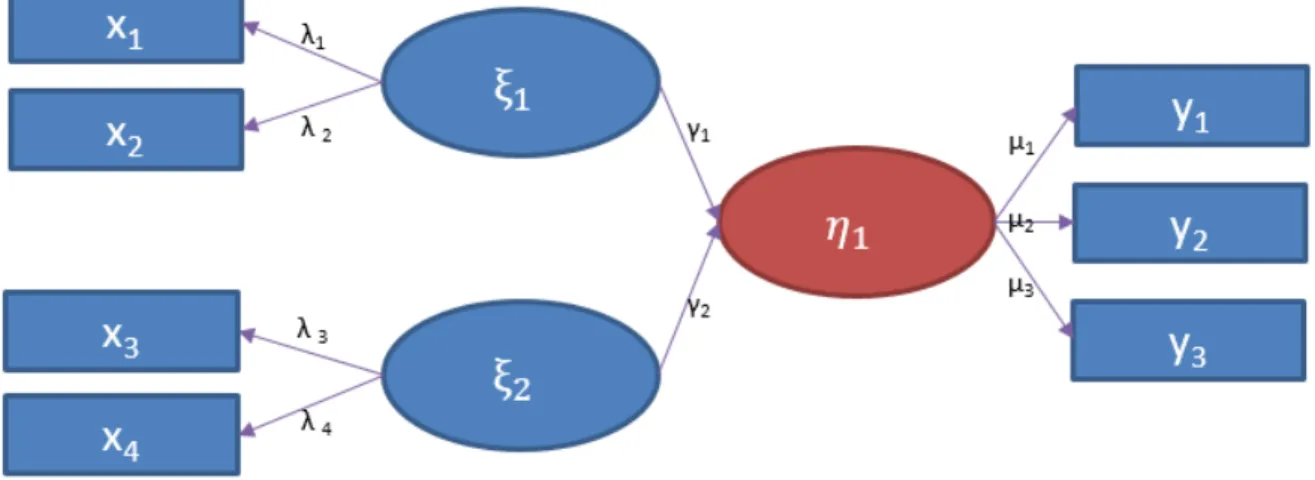
The model structure shown in Fig 2.1 involves one level of measurement model and also one

level of structural model. More levels of measurement model and structural model occur for general SEM modelling. The latent exogenous vector Ξ consists of m latent variables ( , , . . , ), (drawn as blue ellipses in Fig 2.1). The latent endogenous vector (Η) includes

(39)

24

2.1). The measurement variables are represented by the blue rectangles in Fig 2.1.

The basic model includes a number of independent observed variables xi and one dependent

variable y, which are related through several latent variables. One application of this model is to extract the ore-control factors from geo-data. For instance, if xi represents a number of

Fig 2.1 A flowchart showing a simple structural equation model consisting of one level of structure model and one level of measurement model. Rectangle symbols represent observed variables; blue eclipses for latent

exogenous variables and red eclipse for latent endogenous variables.

geochemical elements and y1 represents one variable related with mineralization, the

mineralization related factors in these elements can be estimated by the vector of latent variables, and then mapped through their scores. Another application in geo-data processing is to classify the independent variables xi (i =1, 2, …) under the restriction of dependent variable

(40)

25

measurement model and evaluated by the overall goodness-of-fit of the model.

2.4 CB-SEM and PLS-SEM

As mentioned in Chapter 1, two main approaches for parameter estimation in SEM are CB-SEM and PLS-CB-SEM (Anderson and Gerbing, 1988; Hair et al., 2011; Hair et al., 2012; Hair et al., 2006; Hendry, 1976; James and Singh, 1978; McDonald, 1977; Mehta and Swamy, 1978; Ramsey, 1978; Sargan, 1978; Zellner, 1978). PLS-SEM is one of the commonly used algorithms originally developed by Wold (1966) on the basis of PLS path models and further developed by others (e.g. Hair et al., 2011; Hair et al., 2006). In PLS path models, the explained variances of the endogenous latent variables are maximized by estimating partial model relationships through iterative ordinary least squares (OLS) regression. PLS-SEM is mainly applied in exploratory analysis rather than confirmatory analysis (Hair Jr et al., 2013; Hair et al., 2011; Hair et al., 2006). The estimation procedure for PLS-SEM is an OLS regression-based method while the maximum likelihood (ML) estimation procedure is for CB-SEM. PLS-SEM uses available data to estimate the path relationships in the model by minimizing the errors (i.e. residual variance) of the endogenous constructs. In other words, PLS-SEM estimates the coefficients (i.e. path model relationships) by maximizing the R-square values of the target endogenous constructs. This specific feature achieves the objective of PLS-SEM: prediction. PLS-SEM is, therefore, the preferred method when the research objective is to develop a theory and explain variance (prediction of constructs). For this reason, PLS-SEM is regarded as a variance-based approach to SEM.

(41)

26

Partial least square (PLS) regression is a regression-based approach that explores the linear relationships between multiple independent variables and a single or multiple dependent variables. It differs from the regular regression and constructs composite factors from both of the multiple independent and the dependent variables by means of PCA. PLS regression is particularly useful in predicting a set of dependent variables from a large set of independent variables. It originated in the social sciences (Wold, 1966) but became popular first in chemo-metrics (Geladi and Kowalski, 1986) and in sensory evaluation (Martens and Naes, 1992). But PLS regression is also becoming a tool of choice in the social sciences as a multivariate technique for non-experimental and experimental data processing (Mcintosh et al., 1996). It was first presented as an algorithm akin to the power method but was rapidly interpreted in a statistical framework (Höskuldsson, 1988; Frank and Friedman, 1993; Helland, 1990).

Note that PLS-SEM is similar but not equivalent to PLS regression. PLS regression is a technique that generalizes and combines features from principal component analysis and multiple regressions. PLS-SEM, on the other hand, relies on a pre-specified network of relationships between the constructs as well as between constructs and their measurements. More details about PLS-SEM and PLS can be found in Mateos-Aparicio (2011).

2.5 Remarks

On the ground of the general overview of the SEM, a basic SEM structure is proposed for geo-data processing and analysis, which is a SEM with one level measurement model and one level

(42)

27

structural model. After such a simple model, the measurement model is described in detail as a factor analysis and the structural model is described as a regression model. Although the CB-SEM and PLS-CB-SEM techniques are introduced, PLS-CB-SEM is selected as the algorithm to estimate model parameters in Fig 2.1.

(43)

28

Chapter 3 Dataset and software

3.1 Geological background of study area

The study area, located in Western Meguma Terrain of Nova Scotia, Canada (Fig 3.1), covers

about 25,000 km2_{, and mainly consists of Cambro-Ordovician low-middle grade} metamorphosed sedimentary rocks and a suite of aluminous Devonian granitoid intrusions

(Ryan and Ramsay, 1997; Sangster, 1990). The metamorphosed sedimentary strata of the Meguma Group include two rock formations: the lower sand-dominated flysch Goldenville Formation and the upper shaly flysch Halifax Formation. Both of them were deformed during the Devonian granitoid intrusion emplacement resulting in northeast-southwest trending folds

(Kontak et al., 1998).

The South Mountain Batholith (SMB), which is a complex of multiple intrusions, occupies nearly one-third of the whole study area. Abundant Sn, W, U and Au mineralization and mineral

deposits have been found in this area. While the Sn, W and U mineralization occurs mainly

inside the SMB and in the contact zones between the complex intrusion and the metamorphic sedimentary rocks, the Au deposits occur mainly in the Meguma Group, especially around the

Goldenville and Halifax Contact (GHC) zones (Chatterjee, 1983).

Studies of known Au deposits and their regional geological environment have shown that these

(44)

29

mineralization-related geological features described by previous researchers included GHC, northeast-southwest trending anticline axes and northeast-southwest trending shear zones

(Kontak et al., 1990; Kontak and Kerrich, 1997; Ryan and Ramsay, 1997; Sangster, 1990). Litho-geochemical analyses have shown that As, as a main path-finder element of Au, has

strong but complex relationships with Au mineralization. For example, Au and As are highly

correlated in alteration zones related to Au mineralization controlled by fracture zones or faults

and within the GHC, but not in all gold-bearing quartz veins (Crocket et al., 1986; Kerswill, 1988; Zentilli et al., 1985).

The first regional geochemical survey sampling of the center-lake bottom sediments in Meguma Terrain took place in 1977-1978 and about 4000 samples were collected. The samples were air dried, disaggregated in a ball mill, and sieved to obtain a 20 g portion of the 200 mesh fraction

(Rogers et al., 1985). The collection and quality control methods were described by Garrett et al. (1980). The sampling density was about 1 per 5 km2_{(Rogers et al., 1987)}_{. In 1985, 2950 of} the original samples were reanalyzed for Cu, Pb, Zn, Ag, Li, Rb, Nb, Ti, Sn, Zr, Th, Sb, As, W

and Au. As and Au were detected by the instrumental neutron activity method with a detection

limit of 1 ppm and 5ppb, respectively (Rogers et al., 1987). The study area includes 1948 of the 2950 samples and 1312 of these samples had Au values below the detection limit of 5 ppb; 48

samples had As values below 1 ppm detection limit. The geochemical data from lake sediment

samples have been intensively studied by geochemists who have worked in the area, not only due to the fact that high values of Au, Sn and W partially correspond to known mineral deposits

(45)

30

the main rock units. For example, while F, Li, Nb, Rb, and Sn may reflect existence of granitoid

rocks, Sb, As, Au and W indicate the occurrence of metamorphosed sedimentary rocks

(Bonham-Carter et al., 1988; Dunn et al., 1991; Rogers et al., 1990; Rogers et al., 1987). Distances between the anomalies in lake sediments and their sources were studied in the vicinity of the East Kemptville Sn deposit and surrounding lake basins (Rogers and Garrett, 1987),

which indicated that these have elemental associations similar to those in the bedrock lithogeochemistry. Distances between anomalies in the lake sediments and their sources normally range from several hundreds of meters to several kilometers. The glacial till translation distance in Meguma Terrain ranges from 100 to 1500 m (Graves and Finck, 1988). For regional geochemical research with 1km resolution, the influence of glaciation may not be significant. The bed geologic units are shown in Fig 3.1 and 3.2.

(46)

31

Fig 3.1 The study area in Google earth, the colorful area is the DP ME 132, Version 2, 2006, Regional Lake Sediment Geochemical Survey by the Nova Scotia Department of Natural Resources

(47)

32

(48)

33

Table 3.1 Correlation coefficient between 16 elements in four formations: Goldenville(G), Halifax(H), Granite and Granodiorite (GG), Gneiss and Schist (GS);

Pb All .26 G .22 H .23 GG -.05 GS -.17 Zn All .67 .39 G .54 .41 H .77 .32 GG .31 .21 GS .81 -.16 Ag All .01 .02 .01 G .14 .09 .09 H .05 .13 .03 GG .00 .00 .02 GS -.23 .26 -.36 F All .35 .26 .42 -.01 G .41 .29 .43 -.07 H .30 .20 .39 .07 GG .13 .17 .28 -.03 GS -.27 -.14 -.07 -.46 Li All .41 .39 .58 -.01 .65 G .35 .37 .51 -.07 .79 Halifax .27 .31 .54 .06 .46 GG .18 .37 .50 .00 .53 GS -.38 -.21 -.49 -.15 .33 Nb All .22 .21 .21 .00 .37 .53 G .25 .22 .15 -.04 .60 .66 H .10 .16 .17 .00 .23 .38 GG -.04 .07 -.04 .02 .11 .29 GS .42 .16 .38 -.38 -.27 -.27 Rb All .11 .32 .25 -.03 .53 .72 .43 G .12 .28 .20 -.10 .75 .75 .63 H -.06 .20 .16 -.02 .32 .68 .33 GG -.03 .41 .21 -.02 .43 .77 .25 GS -.15 .11 -.45 .06 -.04 .86 -.10 Sn All .01 .17 .14 .00 .18 .22 .05 .34 G -.02 .19 .17 -.01 .22 .20 .15 .33 H .01 .18 .17 .11 .20 .26 .01 .33 GG -.03 .14 .04 -.03 .12 .25 -.08 .35 GS .57 .20 .32 -.17 -.18 .21 .66 .51 Zr All .02 .23 .12 -.02 .30 .47 .39 .65 .28 G .05 .24 .25 -.04 .57 .63 .57 .72 .38 H -.17 .13 -.05 -.05 .11 .36 .30 .66 .23 GG .05 .32 .20 -.01 .34 .63 .26 .68 .30 GS -.15 .11 -.50 .27 -.21 .76 -.10 .96 .49 Ti All .27 .32 .38 -.02 .49 .71 .56 .60 .22 .67 G .20 .37 .39 -.05 .77 .84 .70 .82 .33 .77 H .05 .21 .18 -.03 .25 .52 .44 .54 .19 .65 GG .24 .21 .39 .00 .39 .66 .32 .41 .13 .60 GS .69 .21 .31 .11 -.22 -.15 .00 .21 .49 .27 Au All .07 .05 .05 .01 .06 .12 .03 .09 .07 .04 .06 G .05 -.01 .06 -.05 .11 .13 .00 .14 .15 .06 .03 H -.01 .10 .00 .04 -.09 -.05 .06 -.06 .00 .01 .04 GG .01 .05 -.10 .06 -.01 .00 -.02 .05 -.04 .01 .02 GS .57 .04 .53 -.27 -.56 -.65 .79 -.45 .29 -.40 .11 Sb All .09 .12 .10 .01 .04 .06 .12 .01 .00 -.03 .05 .10 G .23 .19 .24 .10 .22 .13 .08 .17 .15 .06 .16 .23 H -.03 .05 .01 .03 -.02 -.03 .15 -.09 -.06 -.13 -.08 .12 GG .03 .23 .15 .03 .07 .17 -.01 .08 .06 .13 .22 -.10 GS -.09 .68 .18 .21 -.16 -.25 -.08 -.11 -.08 -.18 -.05 .02 As All .35 .20 .47 .02 .23 .18 .02 .12 .08 .01 .14 .14 .08 G .08 .11 .27 .08 .30 .07 .00 .20 .13 .06 .16 .17 .25 H .60 .23 .63 .14 .16 .18 -.06 -.02 .06 -.11 -.01 .02 -.02 GG .22 .15 .52 .00 .24 .35 -.15 .21 .12 .12 .19 -.05 -.01 GS .93 -.02 .83 -.35 -.12 -.44 .32 -.25 .44 -.28 .73 .52 .04 Th All .51 .35 .65 .01 .55 .73 .45 .57 .19 .53 .62 .07 .11 .30 G .48 .33 .71 -.02 .71 .79 .51 .59 .23 .62 .69 .05 .19 .16 H .49 .27 .60 .07 .41 .58 .30 .45 .16 .34 .41 .03 .07 .40 GG .13 .24 .33 .04 .39 .67 .38 .61 .19 .77 .64 -.02 -.04 .27 GS .07 -.04 -.39 .05 .03 .74 -.10 .90 .54 .88 .43 -.39 -.35 -.06 W All .03 -.01 .02 -.01 .20 .04 .04 .19 .11 .02 .11 .04 .10 .45 .03 G -.01 -.05 -.05 -.03 .33 -.01 .04 .32 .19 .02 .14 .04 .30 .57 .00 H .32 .11 .37 -.05 .14 .18 -.04 .09 .08 .04 .07 -.03 -.05 .33 .13 GG .07 .13 .29 .00 .20 .24 .07 .18 .07 .10 .23 -.09 .19 .34 .19 GS .43 -.49 .58 -.37 -.04 .26 -.10 .17 .18 .08 .17 .01 -.03 .44 .06 Cu Pb Zn Ag F Li Nb Rb Sn Zr Ti Au Sb As Th

(49)

34

(50)

35

3.2 Dataset and transformation

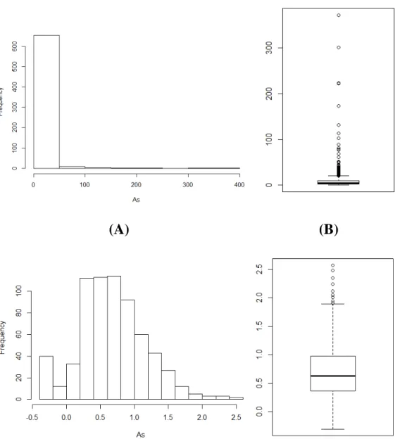
A basic understanding of their statistics is essential for investigating the application of the geochemical dataset used in this research. The samples are grouped into five categories according to the areal geologies: (i) all samples (671), (ii) samples in the Goldenville formation (166), (iii) samples in the Halifax formation (282), (iv) samples in Granite and Granodiorite (GG) rock-type (214), and (v) samples in Gneiss and Schist (GS) rock-type (9). The correlation coefficients between the 16 elements selected for the research in different bedrock geological units in study area are shown in Table 3.1. Since the goal of this research is to find the factors

controlling Au mineralization, the focus tends to be on those elements that are strongly related

to Au. From the correlation coefficients of Au with other 15 elements (Fig 3.5), it is clear that

Au has the highest correlation (0.14) with As. In the other categories, the Au-As correlation

coefficients are: 0.17 (Goldenville), 0.02 (Halifax), -0.05 (GG), and 0.52 (GS). The distribution map of the As (Fig 3.8A) and Au (Fig 3.8B) and other statistical information about the current

dataset including the maximum, minimum, mean and stand deviation of samples are given in

Table 3.2. The log-transformed As and Au are further mapped in Figs 3.8C and 3.8D,

respectively. It can be seen in Fig 3.8B that gold mineral occurrences do not occur in the areas

with high Au concentration values which might be due to: 1) the low accuracy of the data may

not show strong correlation, and 2) the occurrence of mineral deposits may not correspond to high Au concentration values in lake sediments in some locations in the current study area.

(51)

36

Fig 3.4Correlation coefficients between Au and other geo-chemical elements, As has the highest correlation with Au.

Fig 3.5 Correlation coefficients between As and Au in different rock units: the count of samples in each formation are: Goldenville – 166, Halifax – 282, Granite and Granodiorite (GG) – 214, Gneiss and Schist (GS)

– 9; 0.00 0.02 0.04 0.06 0.08 0.10 0.12 0.14 0.16 Cu Pb Zn Ag F Li Nb Rb Sn Zr Ti Sb As Th W ‐0.10 0.00 0.10 0.20 0.30 0.40 0.50 0.60

(52)

37

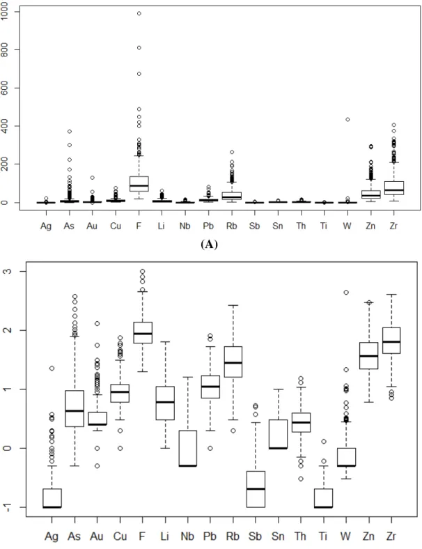
Table 3.2 Statistical analysis of geochemical data

Unit Minimum Maximum Mean Std-Dev

Ag ppm 0.1 22.6 0.23 0.92 As ppm 0.5 372 10.35 25.88 Au ppb 0 130 3.76 6.02 Cu ppm 1 75 10.36 7.11 F ppm 20 990 107.05 78.44 Li ppm 1 63 8.28 8.04 Nb ppm 0.5 16 1.83 2.25 Pb ppm 1 81 12.77 8.42 Rb ppm 2 263 39.05 33.01 Sb ppm 0.1 5.3 0.43 0.82 Sn ppm 1 10 2.18 1.85 Th ppm 0.3 15.3 3.07 1.89 Ti ppm 0 1.3 0.17 0.12 W ppm 0.3 434 1.55 16.77 Zn ppm 6 296 48.24 38.85 Zr ppm 7 406 84.44 62.68

(53)