Revisiting the value of information sharing in two-stage supply chains

This is an Open Access document downloaded from ORCA, Cardiff University's institutional repository: http://orca.cf.ac.uk/111112/

This is the author’s version of a work that was submitted to / accepted for publication. Citation for final published version:

Teunter, Ruud H., Babai, M. Zied, Bokhorst, Jos A.C. and Syntetos, Aris A. 2018. Revisiting the value of information sharing in two-stage supply chains. European Journal of Operational Research

270 (3) , pp. 1044-1052. 10.1016/j.ejor.2018.04.040 file Publishers page: http://dx.doi.org/10.1016/j.ejor.2018.04.040

<http://dx.doi.org/10.1016/j.ejor.2018.04.040> Please note:

Changes made as a result of publishing processes such as copy-editing, formatting and page numbers may not be reflected in this version. For the definitive version of this publication, please refer to the published source. You are advised to consult the publisher’s version if you wish to cite

this paper.

This version is being made available in accordance with publisher policies. See

http://orca.cf.ac.uk/policies.html for usage policies. Copyright and moral rights for publications made available in ORCA are retained by the copyright holders.

# Corresponding author: M. Z. BABAI Kedge Business School

680 cours de la Liberation, 33405 Talence cedex, France

Tel: +33 5 56 84 63 51 ; E-mail: [email protected]

Revisiting the value of information sharing in two-stage supply chains

(Accepted for publication, 24/04/2018, by the European Journal of Operational Research)

1 _{Ruud H. Teunter;} 2,# _{M. Zied Babai;} 1 _{Jos A.C. Bokhorst;} 3 _{Aris A. Syntetos}

1 _{University of Groningen, Faculty of Economics and Business, Nettelbosje 2, 9747 AE Groningen, The Netherlands} 2 _{Kedge Business School, 680 cours de la libération, 33405 Talence Cedex, France}

3 _{Cardiff University, Cardiff Business School, Aberconway Building, Cardiff CF10 3EU, UK} [email protected]; [email protected]; [email protected]; [email protected]

Abstract

There is a substantive amount of literature showing that demand information sharing can lead to considerable reduction of the bullwhip effect/inventory costs. The core argument/analysis underlying these results is that the downstream supply-chain member (the retailer) quickly adapts its inventory position to an updated end-customer demand forecast. However, in many real-life situations, retailers adapt slowly rather than quickly to changes in customer demand as they cannot be sure that any change is structural. In this paper, we show that the adaption speed and underlying (unknown) demand process crucially effect the value of information sharing. For the situation with a single upstream supply-chain member (manufacturer) and a single retailer, we consider two demand processes: stationary or random walk. These represent two extremes where a change in customer demand is never or always structural, respectively. The retailer and manufacturer both forecast demand using a moving average, where the manufacturer bases its forecast on retailer demand without information sharing, but on end-customer demand with information sharing. In line with existing results, the value of information turns out to be positive under stationary demand. One contribution, though, is showing that some of the existing papers have overestimated this value by making an unfair comparison. Our most striking and insightful finding is that the value of information is negative when demand follows a random walk and the retailer is slow to react. Slow adaptation is the norm in real-life situations and deserves more attention in future research - exploring when information sharing indeed pays off.

2

1. Background and motivation

The current backdrop of uncertainty against which supply chains evolve has rendered forecasting and inventory control increasingly challenging tasks. Within this context the bullwhip effect (BE), the phenomenon of order variability amplification as one moves up any given supply chain (Cachon, 2007), is one of the causes of excess inventories in supply chains and low customer service levels. Although the term ‘bullwhip effect’ was first coined by Procter & Gamble in the 1990s, the research that deals with supply chain dynamics and order variance amplification in supply chains dates back to the seminal work of Forester in the late 1960s (e.g. Forrester, 1961; Lee et al., 1997; Chen et al., 2000; Hosoda and Disney, 2006; Boute et al., 2008; Cannella et al., 2013;Mason-Jones and Towill, 2015; Tesfay, 2016). More recently, Fildes et al. (2008) reported that the BE is viewed as one of the most important research areas in the field of Operational Research. For a recent review on the progress and trends of research related to BE, interested readers are referred to Wang and Disney (2016).

Information sharing is one of the most important levers to mitigate the BE in supply chains (Boone and Ganeshan, 2008; Chen and Lee, 2009; Bray and Mendelson, 2012; Dejonckheere et al., 2003; Syntetos et al., 2016). Information sharing refers to the case where some information from a downstream supply chain stage (e.g. a retailer) is available to some upstream stage (e.g. a manufacturer). The supply chain management literature is abundant in discussions on the benefits of demand information sharing (Chatfield et al., 2004; Asgari et al., 2016; Argilaguet-Montarelo et al., 2017). A steady stream of research papers, using mathematical modelling, continues to investigate the conditions under which information sharing is valuable. Chen et al. (2000), Lee et al. (2000), Kim and Ryan, (2003), Ali and Boylan (2011), Cannella et al. (2011), Ciancimino et al. (2012) and Babai et al. (2015) have, among other researchers, shown the value of information

3

sharing in a two-stage supply chain facing stationary Autoregressive Moving Average (ARMA)-type demand processes.

Less has been contributed in this area in the presence of non-stationary demand. Graves (1999), Li et al. (2003, 2005), Zhang (2004) and Gilbert (2005) analysed the properties of orders resulting from a downstream stage facing non-stationary demand under an order-up-to level (OUT) inventory policy. Graves (1999) and Babai et al. (2013) considered a two-stage supply chain where the downstream stage faces Autoregressive Integrated Moving Average (ARIMA) (0,1,1) demand that is forecasted with a single exponential smoothing (SES) method. They showed, numerically and empirically, the potential benefits resulting from forecast information sharing between the retailer and the manufacturer. Interestingly though, their analysis also revealed that for very small values of the smoothing constant, which means that the forecasts react slowly to the demand changes, the benefit of information sharing tends toward zero.

Nevertheless, it should be noted that all previous research in this area has focused on settings where end-customer demand is more indicative of future retailer demand than retailer demand itself. It did so by: (a) assuming that the retailer adapts quickly, maybe even optimally / directly, to any change; (b) often assuming (almost) stationary demand, where changes are indeed not likely to be structural. In addition, in some of the aforementioned research (e.g. Chen et al., 2000; Ali et al., 2012), the authors defined the manufacturer forecast error (upon which the manufacturer safety stock is built) as the difference between its forecast and the end-customer demand, where it should in fact be based on the difference between the forecast and the retailer demand. These assumptions within the literature lead to a wrong evaluation of the real benefit for the manufacturer resulting from information sharing, especially in the case of non-stationary demand processes. This issue constitutes the objective of our work where we revisit some assumptions and findings in the pertinent literature. We do so by means of considering two demand processes: stationary or random walk.

4

These represent two extremes where a change in end-customer demand is never or always structural, respectively. The contribution of this paper is threefold:

1. We revisit/correct the unfortunate upstream stage forecast error definition found in the existing literature and analyse its implications on the value of information sharing.

2. We analyse the value of information sharing under both stationary and non-stationary demand processes in terms of forecast performance and stock control implications.

3. We show that under a random walk demand process, the percentage reduction of the forecast error variance resulting from the use of information sharing is negative which means that there is no value related to information sharing.

The remainder of the paper is organised as follows. In Section 2, we present the assumptions and supply chain structure upon which we theoretically analyse the forecast errors resulting from different information sharing strategies and demand models. Section 3 is dedicated to the analysis of the percentage variance reduction resulting from the use of the information sharing strategy. The stock control implications are discussed in Section 4. The conclusions and natural avenues for further research are presented in Section 5.

2. Assumptions and models

We consider a discrete time model with a single manufacturer and a single retailer. There is a deterministic lead-time � from the supplier (not modelled) to the manufacturer and from the manufacturer to the retailer. We remark that the analysis could be extended to unequal lead-times, but that would make it lengthier and more tedious without providing further insights.

The sequence of events in any period � is as follows. Items shipped by the supplier in period � − � arrive. End-customers demand � items from the retailer. The retailer satisfies demand to the extent possible. The retailer then updates its demand forecast using a simple moving average (SMA) over periods of end-customer demand. The retailer orders from the manufacturer using a base

5

stock policy, where the order-up-to level is selected that gives a − � probability of satisfying lead-time demand (in periods [t + 1,…,� + �]), given the forecast and forecast error distribution. The same applies to the manufacturer, who also forecasts using a moving average over periods (again, to keep the analysis short). Under demand information sharing (DIS), the manufacturer bases its forecasts on end-customer demand. With no information sharing (NIS), the manufacturer bases its forecasts on retailer demand. It is important to remark that the manufacturer must be able to satisfy retailer demand and not end-customer demand with a certain probability, contrary to what is often assumed in the literature (see Section 1).

In the rest of the paper, the following notation will be used.

� Lead-time (both towards the Retailer and the Manufacturer)

Number of periods over which the simple moving average forecast is calculated � End-customer demand in period �

� Retailer order in period �

� _{� Manufacturer order in period � with NIS} �� _{� Manufacturer order in period � with DIS}

� � Retailer order-up-to level in period �

� � _{� Manufacturer order-up-to level in period � with NIS}

��� _{� Manufacturer order-up-to level in period � with DIS}

� Retailer demand forecast in period �

� _{� Manufacturer demand forecast in period � with NIS} �� _{� Manufacturer demand forecast in period � with DIS}

6

� Retailer lead-time demand forecast error in period �

� _{� Manufacturer lead-time demand forecast error in period � with NIS} �� _{� Manufacturer lead-time demand forecast error in period � with DIS}

�� Inverse of the standard normal distribution function at � (safety factor)

In the next two subsections, the system is analysed separately under stationary demand and under demand that follows a random walk, respectively. In both cases, the standard deviation of demand is assumed to be known. This is the standard approach considered in most of the literature that deals with information sharing in supply chains. Moreover, this assumption enables us to compare our findings with those presented in previous work in this area (especially those of Chen et al. 2000) by keeping the experimental framework and all modelling aspects the same. Note that the stationary demand and random walk can be interpreted as two extremes of a spectrum, where a change in demand is always purely by chance for the first case, and always structural and indicative of altered expected future end-customer demand for the second. Real life situations are most likely in between these two cases. Indeed, this explains the popularity of SMA, where an value that is neither too small nor too large results in a ‘reasonable’ performance for all possible situations. This is also the case for SES, where the smoothing constant value can be regulated to result in a robust performance, across a number of possible demand patterns. The choice of SMA in our analysis is quite rational from a practitioner’s perspective. The review of various surveys carried out by Ali and Boylan (2012) shows that SMA was ranked as the top choice in most surveys conducted to ascertain the usage, familiarity and satisfaction of forecasting methods among practitioners. In terms of forecast accuracy, the empirical results from the M1 competition showed that both SMA and SES are associated with very good performance (Makridakis et al., 1982).

7

Before we close this section, it is important to note that our SMA analysis may be easily extended to the use of SES since the derivation process would be along the same lines. Admittedly, we cannot confirm that the conclusions would be the same, but this is broadly what we would expect given that SMA and SES are often treated as equivalent when the average age of the data in the estimates is the same (Brown, 1963).

2.1 Analysis of forecast errors – stationary demand

In this section, we assume that demand � is i.i.d. and Normal with a constant mean  and standard deviation �. We first look at the retailer’s forecast errors and their variance along with the order levels set and the orders placed by the retailer upstream in the supply chain. We then do the same for the manufacturer, distinguishing between the NIS and DIS case.

2.1.1 Retailer

By definition we have

� = ∑=− � − (1)

The lead-time demand forecast error is

� = ∑ � + = − � � = ∑ � + = −� ∑ � − (2) − =

Since end-customer demand is i.i.d. and Normal, the retailer lead-time forecast error is normally distributed with zero mean (unbiased) and variance (see also Prak et al., 2017)

�[ � ] = �� + (�) � = � ( +�) �

So in order to achieve the desired service level �, the retailer order level is set as

8

Note that the latter term in this equation reflects the fact that the forecast differs from the actual mean. Hence, the retailer orders are given by

� = � � − � � − + � = �( � − � − ) + �

Using (1) this can be rewritten as

� = (�) ( � − � − ) + � = ( + �) � −� � − (3) 2.1.2 Manufacturer (No Information Sharing)

Without information sharing, the manufacturer bases its forecasts on the orders placed by the retailer. So we have

� _{� = ∑ � −}

− =

The corresponding lead-time demand forecast error is

� _{� = ∑ � +} = − � � _{� = ∑ � +} = −� ∑ � − − =

Using (3), this can be rewritten in terms of end-customer demands as

� _{� = ( +}�_{) ∑ � +} = − �∑ � + − = − �( + �) ∑ � − − = + (�) ∑ � − − − =

Rearranging the terms and re-indexing them, we further get

� _{� = (}�_{) ∑} �− =�− + − � ∑ �− + =�− + −�( + �) ∑ � =�− + + ( +�) ∑ �+ =�+ (5)

Note that the demand intervals corresponding to the summations in the four terms on the right hand side of (5) are, respectively, [t-2N+1,…,t-N], [t-N+1,…, t-N+L], [t-N+1,…,t], and [t+1,…,t+L]. The

1st_{, 3}rd _{and 4}th _{interval in (5) never overlap. However, the 2}nd _{interval overlaps with the 3}rd _{if �}

and with both the 3rd and 4th interval if < �. Therefore, we proceed by analysing these cases separately.

9

CASE � �

For this case, we get from (5) that

FEMNIS t =(_NL) 2 ∑ D(j) t-N j=t-2N+1 - � + (�) ∑ D(j) t-N+L j=t-N+1 -_NL(1+_NL) ∑ D(j) t j=t-N+L+1 +(1+_NL) ∑ D j t+L j=t+1

Since end-customer demand is i.i.d. and Normal, this retailer lead-time forecast error is normally distributed with mean zero (unbiased) and variance

�[ � _{� ] = (}�_{) � + �} � _{+ (}�_{) � + − �} �_{( +}�_{) � + � ( +}�_{) � �}

CASE � < �

For this case, we get from (5) that

� _{� = (}�_{) ∑} �− =�− + − �+ (�) ∑ � =�− + + ∑ �− + =�+ + ( + �) ∑ �+ =�− + + (7)

Since end-customer demand is i.i.d. and Normal, the retailer lead-time forecast error is normally distributed with mean zero (unbiased) and variance

�[ � _{� ] = (}�_{) � +} � _{+ (}�_{) � + � − � + ( +} �_{) � �}

2.1.3 Manufacturer (Demand Information Sharing)

With demand information sharing, the manufacturer bases its forecasts on the orders placed by the end-customer. So we have

�� _{� = ∑ � −}

− =

The corresponding lead-time demand forecast error is

�� _{� = ∑ � +} = − � �� _{� = ∑ � +} = − � ∑ � − − =

10

Using (3), this can be rewritten in terms of end-customer demands as

�� _{� = ( +}�_{) ∑ � +} = − �∑ � + − = −� ∑ � − − = (8) Similar to the case of NIS, this can be rewritten further as

�� _{� = −}� _∑ � =�− + −� ∑ �− + =�− + + ( + �) ∑ �+ =�+ (9) CASE � �

For this case, we get from (9) that

�� _{� = −} � _∑ �− + =�− + −� ∑ � =�− + + + ( + �) ∑ �+ =�+ (10) and �[ �� _{� ] = � (} �_{) � + − � (}�_{) � + � ( +}�_{) �} = + � (�) � + � ( +�) � � CASE � < �

For this case, we get from (9) that

�� _{� = −} � _∑ � =�− + + ∑ �− + =�+ + ( +�) ∑ �+ =�− + + (11) and �[ �� _{� ] = (} �_{) � + � − � + ( +}�_{) � = (}�_{) � + �� �}

2.2 Analysis of forecast errors - random walk

In this section, we assume that demand follows a random walk process, i.e.

� = � − + � �

where �_� are i.i.d. and Normal with mean 0 and standard deviation �. This can be rewritten as

� = + ∑ ��

11

2.2.1 Retailer

The lead-time demand forecast error is still given by (2). Re-arranging/indexing gives

� = −� ∑ � =�− + + ∑ �+ =�+

From (12) we know that an error term � , � − is ‘included’ in all demand terms in the above equation. Since − + � = , this implies that all error terms � , � − , in the above equation cancel out and we get

� = ∑ (� − � � − + ) � � =�− + + ∑ � + � − + � �+ =�+

Since the error terms are assumed to be i.i.d. and Normal, the retailer forecast error is also Normal. Therefore, as in the case of stationary demand, the variance of the retailer forecast error is constant over time and so is the safety stock. As a result, the retailer orders are still given by (3).

It easily follows from the last equation (by counting the numbers of error terms) that the variance of the forecast errors is given by

�[ � ] = [� + � + � + � − − ] �

2.2.2 Manufacturer (No Information Sharing)

Because (3) still applies, so do all the forecast error expressions that were derived under stationary demand. Note that these are all expressed in end-customer demand terms. What remains, in order to derive the variances under a random walk process, is to rewrite those expressions in error terms � . It easily follows from the general expression (5) that error terms � , � − , always cancel out. In order to obtain the coefficient of � , > � − , we again need to distinguish between the cases � and �.

12

CASE � �

From (6) we get that the coefficients of � in � � are as follows.

Range of Coefficient of � in � � with NIS for �

[� − + , � − ] � − − + (�) − � � + (�) − − � �( + �) + � ( +�) [� − + , � − + �] − � − + � − + � + (�) − − � �( + �) + � ( +�) [� − + � + , �] _{− � − +} �_{( +} �_{) + � ( +}�₎ [� + , � + �] _{� + � − + ( +}� )

Note that for ∈ [� − + , � − ], the term � − − + decreases from to 1, since � is (only) included in , … , � − for this specific range of . For the other ranges of , it similarly holds that the first term of the coefficient of � decreases from the cardinality of that range to 1. So we get �[ � _{� ] =} [ ∑ (�) − � �+ (�) − − � �( +�) + � ( + �) = + ∑ − �+ (�) − − � �( +�) + � ( +�) = + ∑ − �( +�) + � ( + �) − = + ∑ ( + �) = ] � CASE � < �

From (7) we get that the coefficients of � in � � are as follows.

Range of Coefficient of � in � � with NIS for < �

[� − + , � − ] � − − + (�) − �+ (�) + � − + ( +�) [� − + , �] − � − + � + (�) + � − + ( +�) [� + , � − + �] _{� − + � − + + ( +}� ) [� − + � + , � + �] _{� + � − + ( +}�₎

13 So we get �[ � _{� ] =} [ ∑ (�) − � + (�) + � − + ( +�) = + ∑ − � + (�) + � − + ( +�) = + ∑ + ( +�) − = ∑ ( + �) = ] �

2.2.3 Manufacturer (Demand Information Sharing) CASE � �

From (10) we get that the coefficients of � in �� � are as follows.

Range of Coefficient of � in �� � with DIS for �

[� − + , � − + �] − � − + � − + (�) − − � (�) + � ( +�) [� − + � + , �] _{− � − + (}� ) + � ( +�) [� + , � + �] _{� + � − + ( +}�₎ So we get �[ �� _{� ] =} [ ∑ (− (�) − − � (�) + � ( +�)) = + ∑ − (�) + � ( +�) − = + ∑ ( + �) = ] � CASE � < �

From (11) we get that the coefficients of � in �� � are as follows.

Range of Coefficient of � in �� � with DIS for < �

[� − + , �]

− � − + (�) + � − + ( +�)

[� + , � − + �] _{� − + � − + + ( +}�

)

14 So we get �[ �� _{� ] =} [ ∑ (− (�) + � − + ( +�)) = + ∑ + ( +�) − = + ∑ ( + �) = ] �

3. Analysis of the forecast error variance reduction

It is well known and also apparent from the analysis conducted in the previous section that the safety inventory needed to attain a certain service level is positively related to the forecast error variance. Therefore, we analyse the value of information sharing (hereafter denoted by VOI) by considering the (percentage) variance reduction of basing the manufacturer demand forecast on end-customer demand (DIS) instead of retailer demand (NIS).

VOI= �[ � � ] − �[ �� � ]

�[ � _{� ]}

In this section, based on the results of the previous section, we will first derive some analytical results on the sign of the VOI and its behaviour for large N (i.e. forecasts based on many demand observations) under both stationary demand and a random walk. Thereafter, we present numerical results that further illustrate how the VOI depends on the lead-time and N.

Theorem 1:

(a) The VOI is always positive under stationary demand.

(b) The VOI converges to zero if N goes to infinity under stationary demand.

(c) The VOI is negative for a ‘large enough’ N under a random walk and converges to zero if

N goes to infinity.

Proof.

15

�[ � _{� ] > � (} �_{) � + − � (}�_{) � + � ( +}�_{) �} = + � (�) � + � ( +�) � = �[ �� _{� ],}

which implies a positive VOI. Similarly, we get the same result for < � from (7a) and (11a). We can also show that under stationary demand, by developing (6a) and (10a) and using some algebra simplifications, we have

�[ � _{� ] − �[} �� _{� ] =} � � + �

which is always positive.

(b) It easily follows from (6a) and (10a) that under stationary demand, both with and without information sharing, the forecast error variance converges to �� if N goes to infinity, which gives the desired result.

(c) By considering (13) and (14) and using some algebra simplifications, it can be shown that

�[ � _{� ] − �[} �� _{� ] = −}� [� − � + � − + + − + ]_� So lim →∞(�[ � _{� ] − �[} �� _{� ]) = lim} →∞ − � � = −� � <

In addition, since lim

→∞�[

� _{� ] = ∞ , we also have that lim}

→∞� � = , which completes the

proof.

3.1 Numerical analysis

First, we analyse numerically the VOI under different values of N and the lead-time. Figures 1 and 2 show the VOI in the case of a stationary and random walk demand process, respectively, for L = 1, 2, 3, 4 and N ranging from 2 to 40.

16

Figure 1. Numerical results for a stationary demand process: L = 1, 2, 3, 4 and N ∈ [2, 40]

Figure 2. Numerical results for the random walk process: L = 1, 2, 3, 4 and N ∈ [2, 40]

The results in Figure 1 show that under the stationary demand process, VOI is always positive regardless of the value of the lead-time and the N, which confirms what has been shown in Theorem 1. Figure 1 also shows that VOI is a decreasing function of N. So when N increases, the value of

10 20 30 40 10 5 5 L 1 L 2 L 3 L 4 VOI (%) N 10 20 30 40 5 10 15 20 25 30 L 1 L 2 L 3 L 4 VOI (%) N

17

information sharing is reduced. Note that in this case, the moving average with a (very) large N is equivalent to the long term expected demand. However, when the lead-time increases, the value of information sharing increases.

Under the random walk process, Figure 2 shows that the VOI is positive in just a few cases. In fact, VOI is positive only for low values of N, but when N increases (relatively higher than L) VOI becomes negative, which means that when N is relatively higher than L there is no value in sharing information. Figure 2 also shows that VOI is not a monotonic function of the N, which means that there is a maximum percentage reduction of its value (due to the increased variance of forecast error resulting from information sharing) beyond which this reduces and asymptotically tends to zero. In summary, the numerical results in Figures 1 and 2 show that if the retailer is slow to react by using a large N compared to its lead-time from the manufacturer, there is little or no value of information sharing.

4. Stock control implications

In previous sections, we discussed the effects of sharing information on the forecast error variance of the manufacturer. Since forecast error variance is closely linked to the safety stock (needed to attain a certain service level), we expect increased/reduced variance to translate into increased/reduced inventory levels.

However, the exact safety stock calculations are not straightforward to conduct. An important complicating factor is that deliveries from the manufacturer to the retailer are delayed if the manufacturer is out of stock. So, to achieve a certain target service level, the safety stock factor in the order level calculations needs to be larger than what corresponds to a fixed lead-time L. Analytically, dealing with a stochastic delivery time is notoriously difficult, even if the lead-time distribution is assumed to be known. Using approximate safety factors under both NIS and DIS for the same target service level would be unfair when evaluating the VOI, as the achieved service levels

18

might differ. Instead, we consider multiple safety factors consistent with a range of target service levels (0.7, 0.75, 0.8, 0.85, 0.9, 0.95, 0.96, 0.97, 0.98, 0.99) under the assumption of a fixed delivery time L. Using simulation, we then present efficiency curves that trade off the (mean) achieved stock-out probability (i.e. one minus the achieved cycle service level) against the inventory level. The numerical results are generated for a lead-time L = 4; forecasts based on N = 2, 10, 30 observations; mean demand μ = 30; and standard deviation of the demand σ = 10.

The simulation set-up is as follows. The order of events in a period is as described in Section 2, and the order levels are calculated as also described in that section. We allow split/partial deliveries in case the inventory level is not sufficient to satisfy all demand at once. We remark that since lead-time demand forecast errors for future periods are correlated, we base the forecast error variance on ‘lead-time demand error’ observations. In some period t, the most recent lead-time demand error

observation is calculated as the total demand in interval [t-L+1,…,t] minus L times the per period

demand forecast produced in period t-L. The lead-time forecast error variance estimate is then calculated by the sample variance over the last N lead-time demand error observations, just as the forecast itself is based on the last N demand observations. If fewer observations are available during the initial (part of the warm up) phase of a simulation run, then all available observations are used. For any considered setting, we performed 30 runs of 12,000 periods’ length including a warm-up interval of 2000 periods. With regards to the results, we report the average performance between period 2001 and period 12,000. These settings, in conjunction with the information presented in Section 2, facilitates the reproduction (Boylan, 2016) of our results should one wish to do so. We first consider the case where L = 4, N = 10, μ = 30, and σ = 10. Figure 3 shows the efficiency

curves (for the manufacturer) under both NIS and DIS, respectively. Moreover, we present a third ‘DIS (flawed)’ curve whereby manufacturer safety stock levels are based on the forecast error variance of end-customer demand rather than retailer demand. As argued in the introductory section,

19

this is conceptually flawed and leads to an inflation of the VOI. This is confirmed here for the case of inventory levels. For instance, for the largest target service level considered, the flawed logic would suggest a reduction of the inventory level due to information sharing from about 90 to about 50 units, whereas actually still about 80 units are needed to achieve the same service level.

Figure 3. Efficiency curves for the manufacturer under stationary demand: L = 4, N = 10, μ = 30, σ = 10. For ‘DIS (flawed)’, the manufacturer order-up-to level is based on the forecast error variance of the end-customer demand instead of the retailer demand.

In line with previous findings, and with our own analytical results, Figure 3 confirms that, for stationary demand, sharing information consistently reduces inventory levels for the same achieved service. We remark that we also compared efficiency curves for the retailer. However, because they almost overlap for this example and also other examples that will be considered, we decided not to display or discuss them.

Next, we consider the same setting as above except that end-customer demand follows a random walk process. The results are shown in Figure 4.

10 20 30 40 50 60 70 80 90 0.05 0.1 0.15 0.2 0.25 0.3 0.35 0.4 In v e n to ry level (u n its) Stockout probability

Stationary demand,

N

_{= 10}

20

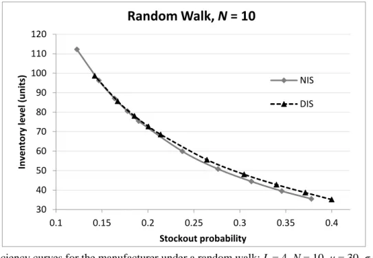
Figure 4. Efficiency curves for the manufacturer under a random walk: L = 4, N = 10, μ = 30, σ = 10

Again, in line with our results, the figure shows that the effect of information sharing is now (slightly) negative for the manufacturer. This confirms that basing order levels on end-customer demand rather than retailer demand under a random walk may deteriorate the performance if the number of observation on which the moving average is based (N) is larger than the lead-time (L). In situations such as the one considered in Figure 4, recent retailer demand is more indicative of forthcoming lead-time retailer demand than recent end-customer demand.

To further demonstrate the effect of the forecast adaption speed under a random walk, we also present the results for N = 2 and N = 30 in Figures 5 and 6, respectively. These confirm that basing manufacturer safety stocks on end-customer rather than retailer demand improves the inventory performance if the speed of adaptation is high but makes it considerably worse if that speed is low.

30 40 50 60 70 80 90 100 110 120 0.1 0.15 0.2 0.25 0.3 0.35 0.4 In v e n to ry level (u n its) Stockout probability

Random Walk,

N

_{= 10}

21

Figure 5. Efficiency curves for the manufacturer under a random walk: L = 4, N = 2, μ = 30, σ = 10

Figure 6. Efficiency curves for the manufacturer under a random walk: L = 4, N = 30, μ = 30, σ = 10

Before we close this section, we should mention that experimentation with other control parameter values leads to similar results (and insights), to those discussed above, and as such are not reported here. 20 40 60 80 100 120 140 160 180 0.1 0.15 0.2 0.25 0.3 0.35 0.4 0.45 Invent or y l evel (u n its) Stockout probability

Random Walk,

N

_{= 2}

Random Walk,

N

_{= 30}

22

5. Conclusion

It is well known that demand variance may be amplified as we move upstream in any given supply chain. For a two-stage supply chain with, for example, a retailer and a manufacturer, this means that the end-customer demand faced by the retailer would typically be less variable than the retailer demand faced by the manufacturer. Consequently, if manufacturers are allowed to have visibility of the downstream less variable demand, they should be able, in principle, to improve their forecasting and inventory performance. That is, demand information sharing is a valuable practice.

Previous studies in this area have demonstrated that this is very often the case. However, some pertinent studies have relied upon an unfair comparison to reach their results. Manufacturers satisfy retailer and not end-customer demand, and as such a manufacturer’s forecasts should be compared (to determine the forecast error) with the demand received by the retailer, rather than the (less variable) demand received by end-customers, which is what previous studies have considered. We find that, for stationary demand (which is the typical setting assumed in the literature) and for a simple moving average forecast method (which is a very popular method in industry, see, e.g., Ali and Boylan, 2012), if the correct comparison is undertaken then the value of information sharing is (much) lower than previously claimed, in terms of inventory performance. Importantly, the inventory levels resulting from a fictitiously reduced forecast error variability lead to a considerable under-achievement of the service levels that manufacturers target to offer to retailers.

We also extend our analysis to the case of non-stationary demand that, apart from a very few studies, has not received much attention. We assume that end-customer demand follows a random walk process whilst forecasting still takes place by means of using a simple moving average method. A striking and insightful finding is that, under this setting, the value of information sharing is negative when the retailer is slow to react to the structural changes (i.e. when the N is large). This is because

23

a change in retailer demand is very likely to be sustained over several periods, making retailer demand itself a better predictor for future retailer demand than end-customer demand.

This clearly shows that focusing on (nearly) optimal forecasting methods that quickly adapt to changes tells only part of the story. Slow adaptation is the norm in real life situations, and deserves much more attention in future research - exploring when collaborative planning and demand information sharing indeed pay off. Future research should also reflect a realistic representation of how inventory systems work, by means of correctly calculating forecast errors and thus safety stock requirements. In light of the results obtained by this work, the pragmatism of the assumptions upon which an information sharing system is built for experimentation purposes appears to be a key determinant of the perceived viability of such system.

Further empirical investigation is also needed. Despite the numerous theoretical claims that demand information sharing offers considerable benefits, it must be acknowledged that empirical case-study evidence in this area is scarce. This paucity of evidence is, partly at least, due to the slow take up of relevant practices in industry (e.g., Syntetos et al., 2016), which in turn raises questions as to why this might have been the case. One would expect a quick take up of something that is valuable and does work and our findings contribute collectively towards some scepticism as to whether this is the case.

References

Ali, M.M., Boylan, J.E. (2011). Feasibility principles for downstream demand inference in supply chains.

Journal of the Operational Research Society, 62: 474-482.

Ali, M.M., Boylan, J.E. (2012). On the effect of non-optimal forecasting methods on supply chain downstream demand. IMA Journal of Management Mathematics, 23: 81-98.

Argilaguet-Montarelo, L., Glardon, R., Zufferey, N. (2017). A global simulation-optimisation approach for inventory management in a decentralised supply chain. Supply Chain Forum: An International Journal, 18:2, 112-119.

24

Asgari, N., Nikbakhsh, E., Hill, A., Zanjirani Farahani, R. (2016). Supply chain management 1982–2015: a review. IMA Journal of Management Mathematics 27: 353-379.

Babai, M.Z., Ali, M.M., Boylan, J.E., Syntetos, A.A., (2013). Forecasting and inventory performance in a two-stage supply chain with ARIMA(0,1,1) demand: theory and empirical analysis. International Journal of

Production Economics, 143: 463–471.

Babai, M.Z., Boylan, J.E., Syntetos, A.A., Ali M.M. (2016). Reduction of the value of information sharing as demand becomes strongly auto-correlated. International Journal of Production Economics, 181: 130-135. Boone, T., Ganeshan, R. (2008). The value of information sharing in the retail supply chain: two case studies.

Foresight: The International Journal of Applied Forecasting, 9: 12–17.

Boylan, J.E. (2016). Reproducibility. IMA Journal of Management Mathematics 27:107-108.

Bray, R., and Mendelson, H., (2012). Information Transmission and the Bullwhip Effect: An Empirical Investigation. Management Science, 58(5): 860-875.

Boute, R.N., Disney, S.M., Lambrecht, M.R., Van Houdt, B. (2008). A win–win solution for the bullwhip problem. Production Planning and Control, 19 (7): 702-711.

Brown, R.G. (1963). Smoothing, forecasting and prediction of discrete time series. Englewood Cliffs, N.J: Prentice Hall, Inc.

Cachon, G.P., Randall, T., Schmidt, G.M. (2007). In Search of the Bullwhip Effect. Manufacturing & Service

Operations Management, 9(4): 457 – 479.

Cannella, S., Barbosa-Povoa, A.P., Framinan J.M., Relvas S. (2013). Metrics for bullwhip effect analysis.

Journal of the Operational Research Society, 64: 1-16.

Cannella, S., Ciancimino, E., Framinan, J.M. (2011). Inventory policies and information sharing in multi-echelon supply chains. Production Planning & Control, 22: 649-659.

Chatfield, D.C., Kim, J.G., Harrison, T.P., Hayya, J.C., (2004). The Bullwhip Effect-Impact of Stochastic Lead Time, Information Quality, and Information Sharing: A Simulation Study, Production and Operations

Management, 13 (4): 340–353.

Chen, F., Drezner, Z., Ryan, J.K., Simchi-Lev, D. (2000). Quantifying the bullwhip effect in a simple supply chain: the impact of forecasting, lead-times, and information. Management Science, 46: 436-443.

Chen, L., Lee, H.L. (2009). Information Sharing and Order Variability Control Under a Generalized Demand Model, Management Science, 55(5): 781 – 797.

Ciancimino, E., Cannella, S., Bruccoleri, M., Framinan, J.M. (2012). On the bullwhip avoidance phase: the synchronised supply chain. European Journal of Operational Research, 221: 49-63.

Dejonckheere, J., Disney, S.M., Lambrecht, M.R., Towill, D.R. (2003). Measuring and avoiding the bullwhip effect: A control theoretic approach, European Journal of Operational Research, 147 (3): 567-590.

25

Forrester, J. (1961). Industrial dynamics. Cambridge, MA: MIT Press.

Hosoda, T., Disney, S.M. (2006). On variance amplification in a three-echelon supply chain with minimum mean square error forecasting. OMEGA: International Journal of Management Science, 34: 344-358. Kim, H.K., and Ryan, J.K., (2003). The cost impact of using simple forecasting techniques in a supply chain.

Naval Research Logistics, 50(5): 388-411.

Lee, H.L., Padmanabhan, V., Whang, S. (1997). Information distortion in a supply chain: the bullwhip effect.

Management Science, 43: 546-558.

Lee, H.L., So, K.C., Tang, C.S., (2000).The value of information sharing in a two-level supply chain.

Management Science. 46: 626–643.

Li G., Wang, S., Yu, G., Yan, H. (2003). The relationship between the demand process and the order process

under a time-series framework. Working Paper. Key Laboratory of Management, Decision and Information

Systems, Chinese Academy of Sciences, Beijing.

Li, G., Wang, S., Yu, G., Yan, H. (2005). Information transformation in a supply chain: a simulation study.

Computers and Operations Research, 32, 707–725.

Makridakis, S., Andersen, A. , Carbone, R. , Fildes, R. , Hibon, M. , Lewandowski, R. , et al. (1982). The accuracy of extrapolation (time series) methods: results of a forecasting competition. Journal of Forecasting, 1 (2), 111–153 .

Mason-Jones, R., Towill, D.R. (2015). Coping with Uncertainty: Reducing “Bullwhip” Behaviour in Global Supply Chains. Supply Chain Forum: An International Journal, 1:1, 40-45.

Prak, D., Teunter, R.H., Syntetos, A.A. (2017). On the calculation of safety stocks when demand is forecasted.

European Journal of Operational Research, 256: 454-461.

Syntetos, A., Babai, Z., Boylan, J.E., Kolassa, S., Nikolopoulos, K. (2016). Supply chain forecasting: theory, practice, their gap and the future. European Journal of Operational Research, 252: 1-26.

Tesfay, Y.Y. (2016). Modeling the Causes of the Bullwhip Effect and Its Implications on the Theory of Organizational Coordination. Supply Chain Forum: An International Journal, 16:2, 30-46.

Wang, X., Disney, S.M. (2016). The bullwhip effect: progress, trends and directions. European Journal of

Operational Research, 250: 691-701.

Zhang X (2004). Evolution of ARIMA demand in supply chains. Manufacturing & Service Operations