Application of Bandelet Transform in Image and Video Compression

(1)

Application of Bandelet transform in

Image and Video compression

Tapan Kiran Adhikari

Department of Electrical Engineering

(2)

Application of Bandelet transform in

Image and Video compression

Dissertation submitted in partial fulfillment

of the requirements of the degree of

Masters of Technology

in

Electrical Engineering

in specialization

Electronic systems and communication

by

Tapan Kiran Adhikari

(Roll Number: 214EE1402)

based on research carried out

under the supervision of

Prof. Dipti patra

May, 2016

Department of Electrical Engineering

(3)

Department of Electrical Engineering

National Institute of Technology Rourkela

Prof. Dipti patra Associate Professor

May 28, 2016

Supervisors’ Certificate

This is to certify that the work presented in the dissertation entitledApplication of Bandelet transform in Image and Video compression submitted by Tapan Kiran Adhikari, Roll Number 214EE1402, is a record of original research carried out by him under our supervision and guidance in partial fulfillment of the requirements of the degree ofMasters of Technology

inDepartment of Electrical Engineering. Neither this dissertation nor any part of it has been submitted earlier for any degree or diploma to any institute or university in India or abroad.

Dipti patra

(4)

Declaration of Originality

I, Tapan Kiran Adhikari, Roll Number 214EE1402 hereby declare that this dissertation entitled Application of Bandelet transform in Image and Video compression presents my original work carried out as a postgraduate student of NIT Rourkela and, to the best of my knowledge, contains no material previously published or written by another person, nor any material presented by me for the award of any degree or diploma of NIT Rourkela or any other institution. Any contribution made to this research by others, with whom I have worked at NIT Rourkela or elsewhere, is explicitly acknowledged in the dissertation. Works of other authors cited in this dissertation have been duly acknowledged under the sections “Reference” or “Bibliography”. I have also submitted my original research records to the scrutiny committee for evaluation of my dissertation.

I am fully aware that in case of any non-compliance detected in future, the Senate of NIT Rourkela may withdraw the degree awarded to me on the basis of the present dissertation.

May 28, 2016

(5)

Acknowledgment

First and foremost, I am truly indebted to my supervisor Professor Dipti Patra for her inspiration, excellent guidance and unwavering confidence through my study. I also thank her for all the gracious encouragement throughout the work. I express my gratitude to the members of Masters Scrutiny Committee, “Professor S. Das, K.R.Subhashini, P. K. Sahoo, Supratim Gupta” for their advise and care. I am also very much obliged to Head of the Department of Electrical Engineering, NIT Rourkela for providing all the possible facilities towards this work. I also thankful to other faculty members in the department for their invaluable support.

My sincere thanks must also go to the members of my thesis advisory: Mr. Yogananda Patnaik, Mrs. Rajashree Nayak, Ms. Smitha Pradhan, Mr Umesh sahu and Mrs. sushree nayak. They generously gave their time to offer me valuable comments towards improving my work.

I am very much grateful to Mr. Yogananda Patnaik for his generous help in particular issues related to simulations. I cannot forget friends who went through hard times together, cheered me on, and celebrated each accomplishment. Thanks for the unforgettable time: L.V Sai Krishna,Satish kumar Reddy Naru,Avinash Buddala and Ajay singh and many others.

My whole hearted gratitude to my parents, “Satyanarayana Adhikari and Jayanti Adhikari’ for their invaluable encouragement and support.

May 28, 2016 NIT Rourkela

Tapan Kiran Adhikari

(6)

Abstract

The need for large-scale storage and transmission of data is growing exponentially With the widespread use of computers so that efficient ways of storing data have become important. With the advancement of technology, the world has found itself amid a vast amount of information. An efficient method has to be generated to deal with such amount of information. Data compression is a technique which minimizes the size of a file keeping the quality same as previous. So more amount of data can be stored in memory space with the help of data compression.

There are various image compression standards such as JPEG, which uses discrete cosine transform technique and JPEG 2000 which uses discrete wavelet transform technique. The discrete cosine transform gives excellent compaction for highly correlated information. The computational complexity is very less as it has better information packing ability. However, it produces blocking artifacts, graininess, and blurring in the output which is overcome by the discrete wavelet transform. The image size is reduced by discarding values less than a prespecified quantity without losing much information. But it also has some limitations when the complexity of the image increases. Wavelets are optimal for point singularity however for line singularities and curve singularities these are not optimal. They do not consider the image geometry which is a vital source of redundancy.

Here we analyze a new type of bases known as bandelets which can be constructed from the wavelet basis which takes an important source of regularity that is the geometrical redundancy.The image is decomposed along the direction of geometry. It is better as compared to other methods because the geometry is described by a flow vector rather than edges. it indicates the direction in which the intensity of image shows a smooth variation. It gives better compression measure compared to wavelet bases. A fast subband coding is used for the image decomposition in a bandelet basis. It has been extended for video compression. The bandelet transform based image and video compression method compared with the corresponding wavelet scheme. Different performance measure parameters such as peak signal to noise ratio, compression ratio (PSNR), bits per pixel (bpp) and entropy are evaluated for both Image and video compression.

(7)

List of Figures

2.1 encoding process . . . 4

2.2 Decoding process . . . 4

2.3 Zig Zag encoder . . . 7

2.4 Basis functions and corresponding tilings of the time-frequency plane : (a) Short-time Fourier transform; (b) wavelet transform. . . 9

2.5 Decomposition process . . . 10

2.6 Composition process . . . 11

2.7 Triangular adaption of an Image geometry . . . 13

2.8 Several different test Images . . . 14

2.9 Comparision of Approximation error decay for different images shown in fig 2.8 . . . 14

3.1 Example of an adapted dyadic squares segmentation of an image and and its corresponding flow . . . 17

3.2 Overview of the algorithm . . . 19

3.3 quadtree segmentation of wavelet space . . . 20

3.4 Zoom of Subsections . . . 20

4.1 Comparision of barb Image Approximation for DCT,DWT and Bandelet Transform . . . 22

4.2 Comparision of lena Image Approximation for DCT,DWT and Bandelet Transform . . . 23

4.3 Comparision of cameraman Image Approximation for DCT,DWT and Bandelet Transform . . . 23

4.4 Comparision of livingroom Image Approximation for DCT,DWT and Bandelet Transform . . . 23

4.5 Comparision of pirate Image Approximation for DCT,DWT and Bandelet Transform . . . 24

4.6 Comparision of mandril Image Approximation for DCT,DWT and Bandelet Transform . . . 24

4.7 Bitrate Vs PSNR of image “barbara”using Bandelet Transform and wavelet transform . . . 25

(10)

4.8 Bitrate Vs PSNR of image “lena”using Bandelet Transform and wavelet transform . . . 25 4.9 Bitrate Vs PSNR of image “cameraman”using Bandelet Transform and

(11)

List of Tables

4.1 Comparison of Approximation of diffterent Images with DCT,DWT and Bandelet Transform methods for Threshold value 0.1 . . . 24 4.2 Comparison of bitrate vs PSNR of different images at different threshold

values . . . 26

(12)

Chapter 1

Introduction

Data compression is necessary for the storage and transmission of images. The use of digital technology and accessing the internet for data transmission is growing exponentially. Without compression, the files will consume a vast amount of memory. For example, a 256 x 256 grayscale image has 65, 536 elements to store. Similarly, a color image stores a million of elements. This large amount of data will take a large amount of bandwidth during transmission, and hence will take a lot of time for downloading or uploading. A large amount of multimedia data consists of images and videos and they occupy a large amount of bandwidth. Hence, the it is necessary to develop an efficient technique for the compression of image and video. It is a common characteristic of images that the neighboring pixels are very much correlated and stores much redundant information. So finding a representation where pixels are less correlated and compact in a place is the basic objective of compression of image and video. For this, we have to remove the redundancy and irrelevancy which in turn will remove redundancy from the image and irrelevant pixels unnoticeable to human eyes. The various image compression standards are JPEG and JPEG 2000.

The above schemes are Discrete Cosine Transform (DCT) [1] based and discrete wavelet transform based. There are issues like blocking artifacts at low bit rates with these schemes. So as to wipe out these issues, scientists have as of late begun examining on wavelets for compression applications. Taking after the determination of wavelets as the principal device for JPEG-2000 (Joint Pictures Expert Group) standard, these endeavors start to develop increasingly [2].

However wavelet transform has also some limitations when the complexity of the image increases. Wavelets are optimal for point singularity however for smooth images these are not optimal. Wavelet bases utilizes sparse approximation which in turn uses some kind of regularity for obtaining value from the neighborhood pixels. But they do not consider an important form of regularity which is geometry. A new class of bases can be constructed from the wavelet bases which takes an important source of regularity that is the geometry called bandelet bases [3].

(13)

1.1 Thesis Organisation

The thesis is Organised as follows

• Chapter 2 is about various Transform techniques such as DCT and DWT and then it explains the Non-linear approximation of Wavelet bases and image representation with geometry.

• Chapter 3 describes about Bandelet Bases,the Fast Discrete Bandelet Transform algorithm and application to image and video compression.

• Chapter 4 is Result and analysis of Image compression of various standard images and Comparison with wavelet basis.

(14)

Chapter 2

Background and Theory

This chapter explains about the different types of compression techniques such as lossy and lossless compression. Various coding techniques such as discrete cosine transform, discrete wavelet transform are described. Then a brief idea about non linear approximation in wavelet basis and the image representation in geometry is described.

2.1 Lossless and Lossy compression

The objective of Image Compression is to represent a picture with a minimal measure of bits conceivable.In Lossy Compression, the picture quality might be degraded to meet a given target of bandwidth for transmission and storage.In lossy coding the picture and video are transmitted through a band limited system. The issue in Lossy Compression is the amount we can lessen the picture quality given the information rate. In Lossy Compression, most methods transform pixels into the transform domain utilizing the DCT (Discrete Cosine Transform) , the DWT (Discrete Wavelet Transform) or Bandelet Transform [4]. The loss is either quantization of the coefficients or the end of the encoding at a given information rate. So as to meet a data rate budget, the transformed coefficients are unequivocally quantized with a given step size as in ZTE, JPEG, H.263 and MPEG-2 . Implicit quantization is utilized as schemes, for example, EZW and SPIHT , which can be truncated anytime in the bit stream amid encoding.

In the lossless compression, the image after decompression is indistinguishable to that of the first. The issue in lossless coding is the amount we can diminish the information rate. The fundamental methodology for lossless image compression is predictive coding or entropy encoding. For predictive coding, DPCM (Differential Pulse Code Modulation) is regularly utilized. For entropy coding, Run-length coding , Huffman coding , or arithmetic coding is utilized. Context modeling can be incorporated into the entropy encoding, which is to measure the likelihood probability of the images molded on the context, to build better compression. The modeling comprises of a mix of neighboring pixels as of now experienced. The structure of predictive coding is controlled by the amount of neighboring pixels utilized for the prediction, weighting for the direct combination of the neighboring pixels

(15)

Chapter 2 Background and Theory

and the strategy for context modeling. The JPEG lossless mode utilizes DPCM and Huffman coding or arithmetic coding . Another strategy for lossless encoding is to utilize the reversible wavelet transform . The consequences of the integer wavelet transform are integers, to recoup the originals totally with the inverse wavelet transform. The lifting scheme (LS) is utilized to execute the integer wavelet transform.

2.2 Image Compression Methods

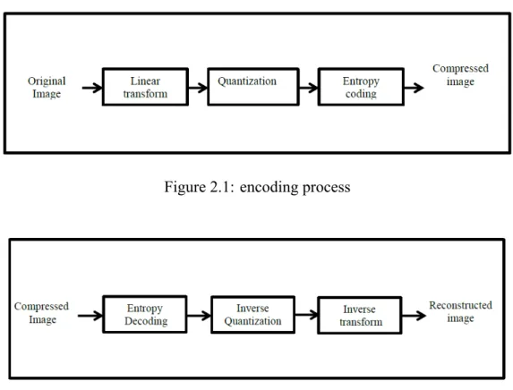
Numerous Image Compression schemes utilize some transform coding. Figure 2.1 demonstrates a block diagram of encoder and decoder utilizing transform coding. The initial step is to get a transform to the image pixels keeping in mind the end goal to lessen the

Figure 2.1: encoding process

Figure 2.2: Decoding process

correlation of the pixels. The aftereffect of the change is known as the transform coefficients. After this progression, in lossy compression, an explicit quantizer might be utilized, or an implicit Quantizer, for example, the truncation of the bit stream might be utilized. The wellspring of the information loss in image compression is the quantizer. In this way, in the lossless compression case, the quantizer is not utilized. The third step is coefficient coding, which implies that the change coefficients are redesigned keeping in mind the end goal to endeavor properties of the transform coefficients and acquire new images to be encoded at the fourth step. For instance, the transform coefficients can be considered as an accumulation of quad-trees or zero-trees and treated in somewhat plane design, to give versatility to the

(16)

compacted bit stream. The images from the coefficient coding are losslessly compacted at the entropy coding step. Entropy coding can be any strategy equipped for packing a succession of symbols, for example, Huffman coding , arithmetic coding and Golomb coding .

2.3 Types of coding techniques

2.3.1 predective coding

For most images, there are redundancies among adjourning pixel values; that is, nearby pixels are very associated. Thus, a current pixel can be predicted sensibly all around given the neighborhood of pixels . The error, which is gotten by subtracting the prediction from the first pixel, has a little entropy than the first pixels. Subsequently, the prediction error can be encoded with fewer bits. In the predictive coding, the relationship between’s contiguous pixels is expelled, and the remaining qualities are encoded. Differential Pulse Code Modulation is known as a predictive coding system.

2.3.2 Transform coding

The goal of image compression is to represent the image pixels with the least number of bits possible. Thus, if the transform coefficients have a small number of non-zero values, they can be represented with a small number of bits . Therefore, the transform needs to compact the energy into the fewest coefficients possible. Due to the property of the orthogonality of the transform, the average squared reconstruction error is equal to the average squared quantization error.

In this scheme, an image is transformed from one domain to a different type of domain, using some well-known transform techniques. Then the transformed values are coded and thus provide greater data compression. Transform coding is an efficient coding scheme based on utilization of interpixel correlation. At first, the pixels in space domain are converted to the frequency domain. Then these coefficients are coded and transmitted. The transform does not achieve any compression, but it helps in decorrelating the data and compacts the significant coefficients into a small data. Like that, many coefficients are omitted after quantization and before encoding.The primary goal of the transform is to make a signal where the signal is less correlated compared to original one. At the receiver; the encoded data are decoded and transformed back to reconstruct the signal.

2.4 Discrete Cosine Transform

The primary objective of The Discrete Cosine Transform is to de-correlate the image information. At that point, the coefficients are encoded. The DCT changes a signal from a

(17)

spatial space into a frequency space. It represents an image as the total sum of the sinusoids of magnitudes and frequencies. DCT has the property that, for a normal image the greater part of the data around an image is packed in only a few coefficients of DCT. After the calculation of DCT coefficients, they are standardized by quantization table with various scales gave by the JPEG standard registered by psycho-visual information. Determination of quantization table influences the entropy and image compression. The estimation of quantization is conversely about nature of the reconstructed image, better mean square error, and better image compression. In a lossy compression procedure, amid a stage called Quantization, the less critical frequencies are disposed of, and afterward, the most essential frequencies that remain are utilized to recover the image in the decomposition process. After quantization, quantized coefficients are modified in a Zig Zag manner for further compressed by an effective lossy coding scheme.The forward DCT can be written as

D(i, j) = √1 2NC(i)C(j) N−1 ∑ y=0 p(x, y)×cos ( (2x+ 1)iπ 2N ) cos ( (2y+ 1)iπ 2N ) (2.1) here, P(x, y) is the input matrix NxN, (x, y) are the coordinate of the matrix elements and (i, j) are the coordinates of the coefficients, and

C(u) = { 1 √ 2f or u= 0 1 f or u >0

The Inverse DCT can be written as

P (x, y) = √1 2NC(i)C(j) N−1 ∑ y=0 D(i, j)×cos ( (2x+ 1)iπ 2N ) cos ( (2y+ 1)iπ 2N ) (2.2) where C(u) = { 1 √ 2f or u= 0 1 f or u >0

2.4.1 Quantization and De-quantization

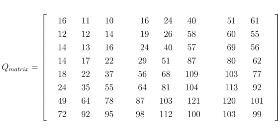
The entire image is partitioned into little N×N squares. At that point working from left to right, start to finish the DCT is applied to every square. Every square’s elements are compressed through Quantization implies isolating by some particular 8×8 lattice called Quantization matrix and adjusting to the closest number quality. This Quantization matrix is chosen by the user to remember that it gives Quality levels extending from 1 to 100, here 1 gives the poor image Quality and most noteworthy image compression while 100 gives the best Quality of decompressed picture and least compression. The standard Quantization

(18)

matrix can be written as

Qmatrix =                 16 12 14 11 12 13 10 14 16 16 19 24 24 26 40 40 58 57 51 60 69 61 55 56 14 18 24 17 22 35 22 37 55 29 56 64 51 68 81 87 109 104 80 103 113 62 77 92 49 72 64 92 78 95 87 98 103 112 121 100 120 103 101 99                

2.4.2 DC and Zig Zag coding

In this step, the quantized coefficients are arranged in a zigzag manner. The DC coefficients are encoded as the difference between DC coefficients of adjacent blocks. Additional compression is achieved by encoding the 63 AC coefficients. There is a strong correlation between pixels of adjacent blocks. This correlation can be removed by arranging them in Zig Zag manner. After arranging, we are getting a stream of frequencies from lower to higher, so that first low-frequency components are arranged then high-frequency coefficients.

Figure 2.3: Zig Zag encoder

2.4.3 Entropy coding

In this section we can achieve loss less compression by Entropy coding which compacts the the Ziz-Zag coded coefficients in a stream of bits. in JPEG [5] entropy coding is achieved by Huffman coding and by Arithmetic coding. it is two step process in which the coefficients of quantization are arranged into a succession of symbols and in the second step we encode the symbols into a stream of data.

(19)

Huffman coding utilizes Huffman table characterized by the application of compressing a picture and after that, the same table is used for decompression. These Huffman tables are predefined or processed particularly for a given image during initialization, preceding compression. Arithmetic coding doesn’t require tables like Huffman coding since it can adjust to the image measurements as it encodes the image. Arithmetic coding is somewhat complicated than Huffman coding for certain execution, for instance, the most high-speed hardware usage. Transcoding between two coding technique is conceivable by essentially entropy decoding with one strategy and entropy recording with the other.

2.5 Wavelet transform

The wavelet transform is orthogonal in nature, similar to Fourier and numerous different transforms utilized as a part of image compression. An orthogonal transform is not only one to one, but the relation is also very simple, due to the spectral theorem.One of the classic tools to achieve different representations of a signal is the Fourier theory, for which a whole set of tools exists in literature: from purely continuous time, such as the Fourier integral, to the Discrete Fourier Transform (DFT) and the Fourier series expansion; moreover, the Fast Fourier Transform (FFT) provides a fast calculation for the transform decomposition. If we are given a pure frequency signalejwt_{, the Fourier-based methods will isolate a peak}

at the frequency w . However, for the simple case of a signal built by k pure oscillations of different frequencies occurring at adjacent intervals in time, we obtain k peaks in the transform domain but the precise time localization is lost. This immediately points out the need for a time-frequency representation of a signal which could give us local information in time and in frequency.

In the Fourier case, the most obvious way to overcome this obstacle is to localize the sinusoids in the transform representation by windowing, that is, the basis functions now become w(t − τ)ejwt_{, where w(t) is a “window” function with small support allowing for time}

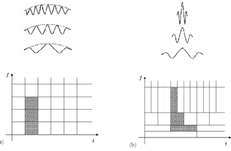
localization. This is traditionally called the windowed Fourier transform, or the short-time Fourier transform (STFT) and was originally introduced by Gabor. By using the concept of the time-frequency plane, it is easy to show that the STFT separates this plane into adjacent square tiles. This is illustrated in the bottom part of Figure 2.4 [6], where the shaded squares in the figure correspond to waveforms which are localized in the same time interval and in three adjacent frequency ranges, as shown in the top part of the figure 2.4.

In the wavelet transform case, a different solution is offered: the precision of the frequency localization is logarithmic, i.e. proportional to the frequency range. Consequently, time localization becomes finer at the highest frequencies. This is illustrated in the bottom part of Figure 2.4(b), and the corresponding wavelets are shown in the figure. It is necessary to look though that one cannot obtain arbitrary localization in time and in frequency due to the uncertainty (Heisenberg) principle [7]. Nevertheless, wavelet theory

(20)

based on multi-resolution analysis and its generalizations offer a natural way to achieve an arbitrary tiling of the time-frequency plane that suits several applications in signal processing [6].

Figure 2.4: Basis functions and corresponding tilings of the time-frequency plane : (a) Short-time Fourier transform; (b) wavelet transform.

2.5.1 Continues wavelet Transform

In wavelet analysis, we use the long time intervals where more precise low-frequency information is required and shorter regions where high-frequency information. Wavelets are orthogonal in nature which means they are periodic signals having average value zero. In Fourier analysis we break up a signal into sine and cosine waves of different frequencies. Similarly, In wavelet analysis we break a signal into scaled versions and shifted versions of the original (or mother) wavelet. In wavelets, the signal is analyzed in time-frequency domain unlike in Fourier theory where sine and cosines are analyzed. The Fourier Transform is the sum over all time of the signal f(t) multiplied by a blurring kernel. The constituent sinusoidal components can be derived from the Fourier transform by multiplying a sinusoidal frequency component. Similarly, in wavelet, the sum of all the scaled and shifted version of the mother wavelet yields the wavelet coefficients. The mother wavelet is given as

ψx,y(a) = 1 √ x� ( a−y x ) ;x, y ∈R andx>0 (2.3) Where a and b are the scaling and shifting parameters respectively. The one dimensional continues wavelet transform can be written as

Wf (x, y) = ∞

∫

−∞X(a)�x,y(a)da (2.4)

(21)

Chapter 2 Background and Theory x(a) = 1 C ∫_∫∞ −∞ Wf(x, y)�x,y(a)dy dx x2 (2.5)

C is the constant and must be finite as it requires one of the property of mother wavelet.

2.5.2 Two-dimensional transform

Since we have quite recently been managing one-dimensional transform in this way, it is not totally clear how to do a two or multi-dimensional transform. There are fundamentally two ways, the easy way, and the difficult way possible. For the most part, the easy way is the quickest and least complex. However, some components in the difficult way possible make it beneficial. To make it basic, we see the image first as columns of one-dimensional flags and change those. At that point we change them in the other heading too. Presently a one-dimensional transform abandons us with a large portion of the coefficients as s. Two-dimensional transform changes both the segments of scaling coefficients and of wavelets, however, there are just the new scaling coefficients in the sections of scaling coefficients, referred to as LL, which is utilized as a part of the following transform. This abandons us with just 1=4 of the underlying information, which means further changes are extraordinarily accelerated. The inconvenience is really finding this information points.

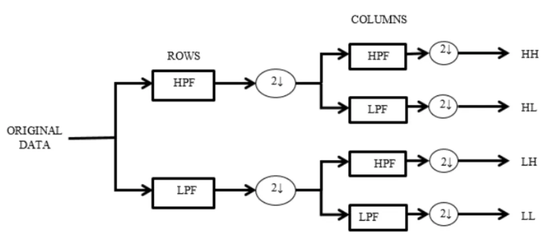
Figure 2.5: Decomposition process

The image is passed through a high and low pass filter along the lines. Consequences of every channel are downsampled by two. The two sub-signals relate to the high and low-frequency parts of the columns, each having a size N by N/2. Each of the sub-signals is on the other hand again passed through high and low-pass filter, yet now along the column and the outcomes are again down-sampled by two. Thus, the first information is part into four sub-sections each of size N/2 by N/2 and contains data from various frequency segments.

(22)

Figure 2.6: Composition process

2.5.3 Non-Linear approximation of wavelet transform

We consider an orthogonal basis B = {gm}m∈N of L

2(_[0_,_1]d)

with for instance d = 1 (signals) or d = 2 (images). We recall that the decomposition of a signal in an orthonormal basis as

f = ∑

m∈z

⟨f, gm⟩gm (2.6)

gives back the original signal and thus produces no error. Processing algorithms modify the coefficients|⟨f, gm⟩| and introduce some error. The simplest processing computes an

approximation by considering only a sub-setIM ∈ Z of M coefficients and performing the

reconstruction from this subset

fM = ∑ m∈IM

⟨f, gm⟩gm (2.7)

WhereIM an index set of M elements, the reconstructed signal isfM is the orthogonal

projection of f onto the space

VM =Span{ψn|m ∈ IM}, (2.8)

Since VM might depend on f, this projectionf → fM might be non-linear. Since the

basis is orthogonal, the approximation error is

||f −fm||2 = ∑ m∈/Im |⟨f, gm⟩| 2 (2.9) The important question is now to choose the setIM , which might depend on the signal f

itself. A non-linear approximation is obtained by choosingIM depending on f. In particular,

(23)

orthogonal, this is achieved by selecting the M largest coefficients in magnitude. This can be equivalently obtained using a thresholding T such that

Im={m ∈ N : |⟨f,gm⟩| >Tm} (2.10)

Where T depends on the number of coefficients M. For discrete pictures of N2 pixels, the same approximations can be actualized in an orthonormal premise B ofN2_{. In compression}

applications, the product of functions is not thresholded but rather quantized and coded. However, it is realized that for a general quantization of step Tm, at huge compression rates the distortion D is relative to||f −fm||2. The bit budget plan R is relative to M. The rate

D(R) in this manner has an asymptotic decay as the guess mistake||f−fm||2as a component

of M. For this applications, given some earlier data on the properties of f, we in this manner need to discover a basis B where||f−fm||2converges rapidly to zero when M increments.

This is the situation if there exist a little steady C and a huge type α then

||f −fm||2 ≤CM−α (2.11)

Wavelet bases have been appeared to be especially proficient for image approximations. A separable wavelet basis is developed from a one-dimensional wavelet Ψ (t) and a scaling function � (t) which are scaled and shifted as

�j,m(t) = 1 √ 2j� ( t−2j_m 2j ) (2.12) and ∅j,m(t) = 1 √ 2j∅ ( t−2j_m 2j ) (2.13) The resulting family of separable wavelets

{∅j,m1(x1)�j,m2(x1) ,�j,m1(x1)∅j,m2(x1) ,�j,m1(x1)�j,m2(x1)}_j_∈_z,₍_m₁_,m₂_∈ _z2₎ (2.14)

Is an orthonormal basis ofL2(R2),To develop a basis over a subset ofR2, one must keep the wavelets whose supports are inside and adjust suitably the ones whose supports meet the limit of Ω. we might in any case composeϕj,m andψj,mthe adjusted scaling functions and

wavelets at the limit, and the subsequent basis ofL2₍₎_{can be composed as}

{∅j,m1(x1)�j,m2(x1) ,�j,m1(x1)∅j,m2(x1) ,�j,m1(x1)�j,m2(x1)}₍_j,m₁_,m₂₎_∈_I_� (2.15)

On the chance that the discrete imagef(x1, x2)is consistently regular and if the wavelet

ψ has p > α vanishing moments then estimatefmfrom M wavelets fulfills

||f −fm||2 ≤CM−α (2.16)

(24)

2.5.4 Geometrical representation

In spite of the optimality of wavelets for limited variation functions, one can frequently enhance the estimation performance of wavelet bases for pictures, by watching that the level arrangements of numerous images have a finite average as well as are regular geometric curve. using this geometric normality can permit us to enhance the representation. This can be shown by a basic example. Let us consider a set of[0,1]2 whose limit is a piecewiseC2

curve, with a limited number of corners.Assume thatf(x1, x2)is aC2 capacity inside and

outside, which is intermittent along the boundary. One can confirm that there exist C1 and C2 such that the wavelet estimatefm fulfills

C1M−1 ≤ ||f−fm||2 ≤C2M−1 (2.17)

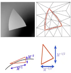
This can be enhanced with representations adjusted to the picture geometry. A basic

Figure 2.7: Triangular adaption of an Image geometry

case is found with a piece-wise linear estimate developed over an adapted triangulation represented in Figure 2.7. The limit is secured with thin triangles whose widths areO(M−2), and within and outside of are secured by extensive triangles so that the aggregate number of triangles is M. Over such a triangulation, one can develop a piecewise straight estimation

fm fromf that fulfills

||f −fm||2 ≤C2M−2 (2.18)

Here the decay rate exponent α = 2 which is superior than with wavelets, and this estimation decay is similar to the one obtained whenf is C2 _{over its whole support. The}

presence of discontinuities does not degrade the asymptotic decay of the estimation.

This case demonstrates that utilizing the geometrical image redundancy can prompt much littler approximation mistakes for an fixed number of estimation components M. One should likewise incorporate the way that these estimation components (triangles) are characterized by numerous parameters (orientations, width, length), which can be fused in the constant C

(25)

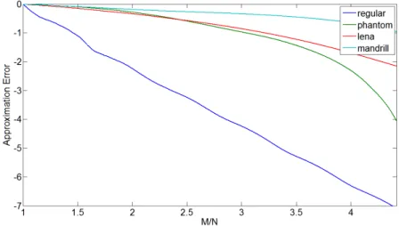
Figure 2.8: Several different test Images and which does not influence the asymptotic decay rate.

2.5.5 Comparision of signals

For a fixed basis (for instance wavelets), the decay of||f−fm||2 allows one to compare the

complexity of different images.

Figure 2.9: Comparision of Approximation error decay for different images shown in fig 2.8 Figure 2.8 shows that natural images with complicated geometric structures and textures are more difficult to approximate using wavelets. Since the approximation error often decays in a power-low fashion , the curves are displayed in a log-log plot in figure 2.9.

(26)

Wavelets are optimal for point singularities in natural images but for smooth cartoon images it is not optimal. As complexity increases wavelet performance decays. Hence, geometrical regularity can give a better approximation. Bandelets are a new basis to approximate the ideal transform. These bases take an important form of redundancy i.e. geometry and hence the error decay can be faster as compared to wavelet bases for smooth images.

(27)

Chapter 3

Bandelet Transform based Image and

video compression

Bandelet bases are new class of bases which decompose the image in the direction of geometric flow. The image gray levels have regular variations along the geometric flow. A fast subband filtering algorithm is implemented for the decomposition of the image. Geometrically regular images have optimal approximation rates for bandelet bases. A fast best basis algorithm is used for optimizing the bandelet basis geometry in case of image compression.

sparse representations are utilized for the precise approximation of signal with few parameters in case of compression application or noise removal [4].these schemes predict values from their neighbors by taking advantage of some regularity. Representations in orthonormal bases have been shown to be particularly efficient for images and having wavelet bases and cosine bases. They are having square support and can be constructed with separable products of one-dimensional basis. these bases do not consider the geometric regularity which is a vital source of redundancy.but representation of edges are difficult as they have sharp transitions and hence they are costlier.

The bandelet bases can be constructed as a field of vectors which are parallel to the direction of flow along which image intensities are changing regularly. We call this vector field as geometric flow. This flow vector can be optimized based on the application which is a challenging task.wavelet bases are warped along the flow vector for finding out the bandelet bases.this method is called bandeletization.

3.1 Bandelets along geometric flow

Rather than portraying the image geometry through edges, which are frequently not well characterized, the geometry of image is described by a field of vectors which locally give a direction where the image has regular variations. This vector field is known as a geometric flow.

(28)

Chapter 3 Bandelet Transform based Image and video compression

3.1.1 Bandelet Basis

This segment depicts the development of bandelet bases from wavelet bases that is twisted along the geometric curve, to exploit the image redundancy along this stream. Conditions are forced on the geometric curve to acquire orthonormal bandelet bases. In an area Ω, a geometric stream is a vector field τ(x1, x2)characterized at each τ(x1, x2) ∈ Ω, which

shows locally a heading in which the image force f has regular variations. In the event that the image intensity is consistently regular in the area of neighborhood a point then this course is not extraordinarily characterized. Some type of normality is in this way forced on the curve to determine it. To develop orthogonal bases with the subsequent flow, a first normality condition forces that the flow is either vertically parallel , which implies thatτ(x1, x2) =

τ(x1), or horizontally parallel and thusτ(x1, x2) =τ(x2). To keep up enough adaptability,

this parallel condition is forced inside sub rigions of the image support. The image S is divided into sub rigionsS=UiΩiand inside each the flow is either parallel on a level plane

or vertically. On the off chance that the image intensity f is consistently general over an entire rigion then a geometric stream is insignificant and is in this manner not characterized.

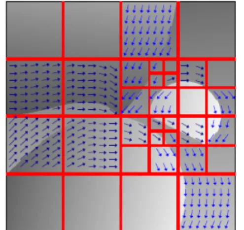
Figure 3.1: Example of an adapted dyadic squares segmentation of an image and and its corresponding flow

In the fig 3.1 we can see that the image intensities are regularly varying along the curves. so we can apply a wavelet transform by warping up the vectors in these directions so that the anisotropy which is not removed can be easily removed. This can be done by applying a Bandeletization method which calculates the direction d weather parallel to horizontal curve or vertical curve and applies a inverse warping operation in each sub square.

(29)

3.2 Application to Image Compression

The correlation near the singularity of a wavelet coefficient can be removed with the help of bandeletization method [8]. There must be some regularity in the transformed surface for removing this redundancy. The following two source of regularity can be implemented.

3.2.1 Regularity due to the wavelet transform

Whenever we perform a 2-d wavelet transform to an image most of the redundancy is removed but the anisotropy near the singularity is not getting removed. however if it is found that along the orthogonal direction of the anisotropy the image intensities are varying regularly. hence there is a regularity along perpendicular direction of the anisotropy.

3.2.2 Regularity due to the Geometry

It is found that if we move along the direction of geometry the image intensities are smoothly varying. So if we can re arrange the pixel values of high singularity and reorder them we can able to compress the anisotropy which is not removed by the wavelet transform.

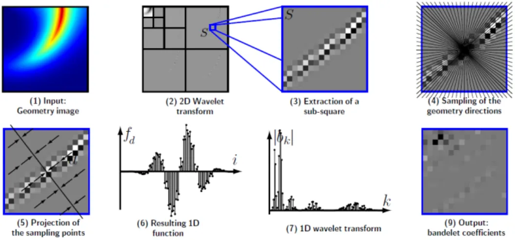
3.2.3 Bandletization

Reordering of the grid points(step1)

In this section we first apply a 2 dimensional wavelet transform and try to remove the anisotropy which is not removed by the regularity due to wavelets. A square is selected and of width L.we use directional projection to project the points on to the direction which is orthogonal to the geometry. Then new points will be generated. Then we select every sampling locations and project them into the perpendicular direction. These points now are re ordered from left to right so that we will get a new 1 dimensional signal.

1D wavelet Transform(step2)

In this section we will apply a 1 dimensional wavelet transform to the resulting signal from the previous section so that we can compress it by removing the anisotropy. we will select a threshold value T and remove all the coefficients which are less than the specified value. This method we will apply for every square s and for every direction d. We can find the best direction by minimizing the approximation error between the original signal and the reconstructed signal.

(30)

3.3 Fast Discrete Bandelet Transform Algorithm

The following are the steps for Bandelet Transform algorithm. • an input image is provided and a threshold is defined.

• Then a 2 dimensional orthogonal wavelet transform is computed along the horizontal, vertical and diagonal direction. Then step 3-7 are repeated for each each of the transform.

Figure 3.2: Overview of the algorithm

• The wavelet transformed image is partitioned into subsquares of equal size, and a dyadic square is obtained of width L pixels.the steps 4-7 is repeated.

• then the sun space is sampled into as many as number of direction possible which is generally2L2. Each of the direction is selected and step 5-7 are repeated.

• The sampling locations are projected along the direction d and the result is sorted from left to right.

• This re ordering gives us a 1 dimensional discrete signal. • Then a 1 d discrete wavelet transform is carried out.

• The best direction is chosen from all the direction which gives least approximation error for a given threshold T.This can be done by minimizing the Lagrangian L. • Then the output is stored as a 2 dimensional image. A arithmetic coding is done to

ensure that the low frequency components are placed in the left corner where as the high frequency components in the right most corner.

• After computing the approximation we have to choose the best approximation squares which can be done by building a quad tree.

(31)

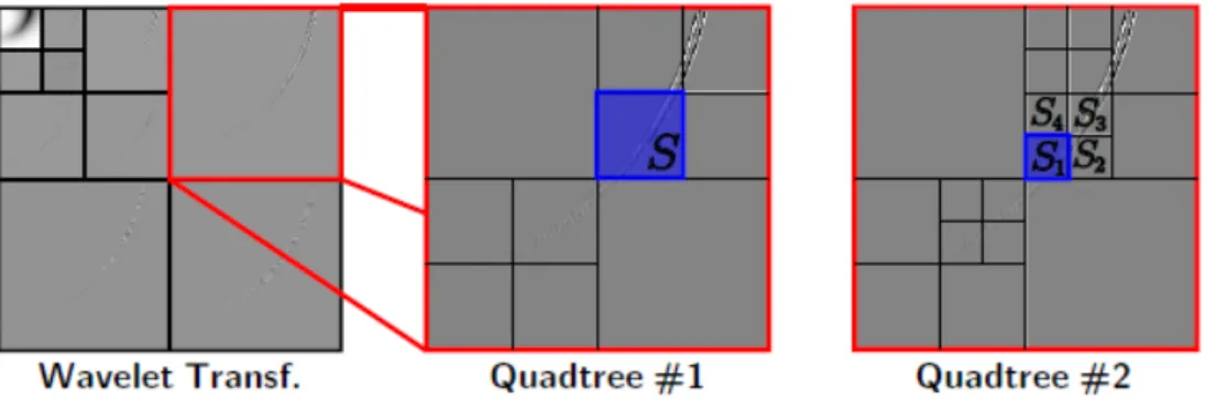
3.3.1 Quadtree construction

While building a quadtree only one sub square is chosen and the coefficients of other squares are discarded. figure 3.3 and 3.4 shows two different quadtrees of finest scale

2j_.

Figure 3.3: quadtree segmentation of wavelet space

Figure 3.4: Zoom of Subsections

After we chose a segmentation for each finest scale2j _{and an approximate direction}

of geometry d inside every square, we can write the bandelet basis asX = {bm}m

, where m is the indexing parameter of the basis vector. The bandelet transform computes the dot products i.e. the projection of a function f on this basis,{⟨f, bm⟩}m

. Thus a bandelet projection consists A quadtree segmentation for each scale2j . For each dyadic square and for each scale in the quadtree, the direction of geometry d, the bandelet coefficients{⟨f, bm⟩}. wherever in the sub square the image is regular,

which means there is no geometry. In those cases we can keep the original wavelet coefficients.

3.4 Application to Video Compression

Here our aim is to construct a single bit stream which can be applicable to different resolution devices. For example, a mobile may need a lower resolution video as compared to a digital

(32)

TV. Here we generate a bit stream which can decoded by both mobile and TV as per the requirements. In this thesis, we have tried to compress the video based on bandelet transform. Our initial attempt was to implement spatially scalable video compression. Later we extended it with few changes for quality (PSNR) scalability. Core part of the model is based on set partitioning in hierarchical tree (SPIHT) algorithm. The further content is removed for publication purpose.

(33)

Chapter 4

Result and Analysis

4.1 Result and analysis for Image compression

The final image code is obtained by decomposing the image in the bandelet basis associated to the optimized partition and its geometric flow. To evaluate the performance of this bandelet compression algorithm, we compare the PSNR of the Bandelet Transformed Image with the PSNR of Haar wavelet basis,and with the DCT approximation basis with the same quantization and entropy coding procedure. We do not incorporate the bit-plane strategy and the contextual coding procedure of JPEG-2000 to compare more easily the performance of the bandelet and wavelet bases themselves. Similar bit plane and contextual coding procedure can also be applied to bandelet coefficients.

Figure 4.1: Comparision of barb Image Approximation for DCT,DWT and Bandelet Transform

Figure 4.1 shows the approximation of Barbara image with DCT, DWT and Bandelet transform techniques. At first the image is Transformed with different methods. Then the image is quantized with threshold value of 0.1 and again reconstructed with inverse Transform method. Entropy coding scheme is not applied in this procedure.Different Compression parameters such as Peak Signal to Noise Ratio (PSNR), Compression Ratio (CR), No. of Bit (bpp), Entropy were derived from the three techniques. It is found that the Bandelet approximation method outperforms the corresponding DWT and DCT schemes by 1.2 dB and 2.8 dB respectively. Similarly it is done for different standard Images. Table 4.1

(34)

Chapter 4 Result and Analysis

Figure 4.2: Comparision of lena Image Approximation for DCT,DWT and Bandelet Transform

Figure 4.3: Comparision of cameraman Image Approximation for DCT,DWT and Bandelet Transform

Figure 4.4: Comparision of livingroom Image Approximation for DCT,DWT and Bandelet Transform

shows a whole comparison of all the parameter and Bandelet scheme performance is superior in all the cases.

Figure 4.7, 4.8, 4.9 shows the distortion rate curves for Barbara, lena and Cameraman Images. fifteen threshold values were taken and the bit rate is calculated for both bandelet and wavelet scheme.from the curves it is found that the bandelet coder outperforms the wavelet coder. It is important to observe that this remains valid for a bit rate going from .15 bit per pixel to 1 bit per pixel, which covers the whole range of applications. From a visual quality

(35)

Figure 4.5: Comparision of pirate Image Approximation for DCT,DWT and Bandelet Transform

Figure 4.6: Comparision of mandril Image Approximation for DCT,DWT and Bandelet Transform

Table 4.1: Comparison of Approximation of diffterent Images with DCT,DWT and Bandelet Transform methods for Threshold value 0.1

Images Method PSNR CR No. of Bits(bpp) Entropy Lena DCT 23.0251 2.8 0.878 0.88 DWT 25.7915 4 0.72 0.719 Bandelet Transform 26.8192 4.2 0.7 0.707 barbara DCT 23.8601 2.3 0.999 1 DWT 25.4888 3.8 0.767 0.77 Bandelet Transform 26.6644 3.9 0.723 0.72 Cameraman DCT 23.411 2.3 1 1 DWT 26.6008 4.3 0.678 0.68 Bandelet Transform 27.7083 4.42 0.663 0.66

point of view, the difference of performance between the two coders is more impressive. It can be seen from the Table 4.2 that the Bandelet coder PSNR for Barbara image is 1.4 dB

(36)

Figure 4.7: Bitrate Vs PSNR of image “barbara”using Bandelet Transform and wavelet transform

Figure 4.8: Bitrate Vs PSNR of image “lena”using Bandelet Transform and wavelet transform

more than the corresponding wavelet coder where as for Lena and cameraman it is 0.8 db and 1.1 dB approximately.Eventhough the bandelet coder introduces errors, the restored images have a regular geometry along the direction of the computed flow, and the resulting error is hardly visible.

On the contrary, wavelets introduce visible ringing effects that are distributed the square grids of the wavelet sampling, which partly destroys the geometrical regularity. As a result, the bandelet compressed images have a better visual quality than their wavelet counterparts.

(37)

Figure 4.9: Bitrate Vs PSNR of image “cameraman”using Bandelet Transform and wavelet transform

Table 4.2: Comparison of bitrate vs PSNR of different images at different threshold values Images Threshold Bitrate wavelet Bitrate Bandelet PSNR Wavelet PSNR Bandelet Barb 0.1 0.6391 0.7191 31.4576 32.8732 0.3 0.1689 0.2273 25.6994 27.0901 0.5 0.0565 0.1200 23.8128 24.4591 0.7 0.0270 0.0744 22.1868 23.7449 Lena 0.1 0.5802 0.7057 31.5822 32.1447 0.3 0.1464 0.2099 26.0586 26.6989 0.5 0.0710 0.1049 23.8826 24.5342 0.7 0.0424 0.0581 22.7794 23.0772 Cameraman 0.1 0.5747 0.7017 31.8699 32.9082 0.3 0.1651 0.2486 26.9734 27.6777 0.5 0.0777 0.1085 24.9052 25.0660 0.7 0.0484 0.0649 23.7676 24.6557

The main inefficiency of the current bandelet scheme comes from boundary effects between regions having different geometric flow. We use a bandelet transform that includes vectors that go across regions and thus produces no compression artefacts at the boundary of such regions.

(38)

4.2 Result and analysis for video compression

For video compression CITY and FOREMAN sequences are taken and compression is performed. The further content is removed for publication purpose.

4.3 Conclusion

In this thesis, we carried out image and video compression using a new class of bases known as bandelet bases. We took some standard images and approximated them using discrete cosine transform, discrete wavelet transform, and bandelet transform. Then different compression measures were evaluated and wrote it down in tabular form. In every case, the bandelet transform based coder outperforms the DCT and DWT based coder. Curves were plotted for different threshold values which show optimality of bandelet transform over wavelet transform. Similarly, several standard video sequences were taken and compared with the corresponding wavelet-based coder and results are noted down. The bandelet based video compression scheme shows the good result as compared to the wavelet-based coder. For video image sequences, a three-dimensional time-space geometric flow can be defined to construct bandelet bases that are adapted to the space-time geometry of the sequence.

(39)

References

[1] K. R. Rao and P. Yip,Discrete cosine transform: algorithms, advantages, applications. Academic press, 2014.

[2] S. G. Mallat, “A theory for multiresolution signal decomposition: the wavelet representation,”Pattern

Analysis and Machine Intelligence, IEEE Transactions on, vol. 11, no. 7, pp. 674–693, 1989.

[3] E. Le Pennec and S. G. Mallat, “Geometrical image compression with bandelets,” in Visual

Communications and Image Processing. International Society for Optics and Photonics, 2003, pp.

1273–1286.

[4] E. Le Pennec and S. Mallat, “Sparse geometric image representations with bandelets,”Image Processing,

IEEE Transactions on, vol. 14, no. 4, pp. 423–438, 2005.

[5] G. K. Wallace, “The jpeg still picture compression standard,”Consumer Electronics, IEEE Transactions on, vol. 38, no. 1, pp. xviii–xxxiv, 1992.

[6] M. Vetterli and C. Herley, “Wavelets and filter banks: Theory and design,” Signal Processing, IEEE

Transactions on, vol. 40, no. 9, pp. 2207–2232, 1992.

[7] I. Daubechies, “The wavelet transform, time-frequency localization and signal analysis,” Information

Theory, IEEE Transactions on, vol. 36, no. 5, pp. 961–1005, 1990.

[8] G. Peyré and S. Mallat, “Surface compression with geometric bandelets,”ACM Transactions on Graphics

(TOG), vol. 24, no. 3, pp. 601–608, 2005.

Application of Bandelet Transform in Image and Video Compression

Application of Bandelet transform in

Image and Video compression

Tapan Kiran Adhikari

Department of Electrical Engineering

Application of Bandelet transform in

Image and Video compression

Masters of Technology

Electrical Engineering

Electronic systems and communication

Tapan Kiran Adhikari

Department of Electrical Engineering

Department of Electrical Engineering

National Institute of Technology Rourkela

Supervisors’ Certificate

Declaration of Originality

Acknowledgment

Abstract

Contents

List of Figures

List of Tables

Chapter 1

Introduction

1.1

Thesis Organisation

Chapter 2

Background and Theory

2.1

Lossless and Lossy compression

2.2

Image Compression Methods

2.3

Types of coding techniques

2.3.1

predective coding

2.3.2

Transform coding

2.4

Discrete Cosine Transform

2.4.1

Quantization and De-quantization

2.4.2

DC and Zig Zag coding

2.4.3

Entropy coding

2.5

Wavelet transform

2.5.1

Continues wavelet Transform

2.5.2

Two-dimensional transform

2.5.3

Non-Linear approximation of wavelet transform

2.5.4

Geometrical representation

2.5.5

Comparision of signals

Chapter 3

Bandelet Transform based Image and

video compression

3.1

Bandelets along geometric flow

3.1.1

Bandelet Basis

3.2

Application to Image Compression

3.2.1

Regularity due to the wavelet transform

3.2.2

Regularity due to the Geometry

3.2.3

Bandletization

3.3

Fast Discrete Bandelet Transform Algorithm

3.3.1

Quadtree construction

3.4

Application to Video Compression

Chapter 4

Result and Analysis