Mutual Information and Conditional Mean Prediction Error
Clive G. Bowsher1 and Margaritis Voliotis School of Mathematics,
University of Bristol, U.K.
Abstract
Mutual information is fundamentally important for measuring statistical dependence between variables and for quantifying information transfer by signaling and communication mechanisms. It can, however, be challenging to evaluate for physical models of such mechanisms and to estimate reliably from data. Furthermore, its relationship to better known statistical procedures is still poorly understood. Here we explore new connections between mutual information and regression-based dependence measures, ν−1, that utilise the determinant of the second-moment matrix of the conditional mean prediction error. We examine convergence properties as ν→0 and establish sharp lower bounds on mutual information and capacity of the formlog(ν−1/2). The bounds are tighter than lower bounds based on the Pearson correlation and ones derived using average mean square-error rate distortion arguments. Furthermore, their estimation is feasible using techniques from nonparametric regression. As an illustration we provide bootstrap confidence intervals for the lower bounds which, through use of a composite estimator, substantially improve upon inference about mutual information based onk-nearest neighbour estimators alone.
Index Terms
Lower bound on mutual information, relative entropy, information capacity, nearest-neighbour estimator, corre-lation and dependence measures, regression.
I. INTRODUCTION
Mutual information is fundamentally important for measuring statistical dependence between variables [1], [2], [3], [4], and for quantifying information transfer by engineered or naturally occurring communication systems [5], [6]. Statistical analysis using mutual information has been particularly influential in neuroscience [7], and is becom-ing so in systems biology for studybecom-ing the biomolecular signalbecom-ing networks used by cells to detect, process and act upon the chemical signals they receive [8], [9], [10]. It can, however, be challenging to estimate mutual information reliably with available sample sizes [11], and difficult to derive mutual information and capacity exactly using mechanistic models of the ‘channels’ via which signals are conveyed. Furthermore, connections between mutual information and better known statistical procedures such as regression, and their associated dependence measures, are still poorly understood. In order to address these challenges, the relationship between mutual information and the error incurred by estimation (or ‘prediction’) using the conditional mean is now receiving attention. The focus has been on minimum mean square estimation error or, more generally, its average across the elements of the vector being estimated [12], [13], [14]. Instead, we focus on connections between mutual information and regression-based dependence measures, ν−1, that utilise the determinant of the second-moment matrix of the conditional mean prediction error. We examine convergence properties as ν →0, and establish sharp lower bounds on mutual information of the form log(ν−1/2). The bounds are tighter than lower bounds based on the Pearson correlation and ones derived using average mean square-error rate distortion arguments.
Themutual informationbetween 2 random vectorsXandZ, writtenI(X;Z),is the Kullback-Leibler divergence between their joint distribution and the product of their marginal distributions [15]. Mutual information thus measures the divergence between the joint distribution of (X, Z)and the distribution in which X andZ are independent but have the same marginals. I(X;Z) has desirable properties as a measure of statistical dependence: it satisfies (after monotonic transformation) all 7 of R´enyi’s postulates [16] for a dependence measure between 2 random variables, and underlies the recently introduced maximal information coefficient [4] for detecting pairwise associations in large data sets. Importantly, mutual information captures nonlinear dependence and dependence arising from moments higher than the conditional mean.
A decision-theoretic interpretation is indicative of the broad applicability of mutual information as a summary measure of statistical dependence. It can be shown [17] thatI(X;Z)is equal to the increase in expected utility from
1
corresponding author: [email protected]
reporting the posterior distribution of either of the two random vectors based on observation of the other, compared to reporting its marginal distribution—for example, reportingp(Z|X=x)instead ofp(Z). This holds when the utility function is a smooth, proper, local score function—as appropriate for scientific reporting of distributions as ‘pure inferences’ [18]—because the logarithmic score function is the only score function having all these properties. In information theory, the supremum ofI(X;Z)over the set of allowed input distributions F, termed theinformation capacity, equates to the maximal errorless rate of information transmission over a noisy channel when the channel is used for long times [5].
The above discussion makes clear that, from a rich variety of perspectives, mutual information is fundamentally important for measuring statistical dependence and for quantifying information transfer by signaling and commu-nication mechanisms.
Our general setting may be depicted as
X→Y →Z, (1)
with (X, Y, Z) a real-valued random vector. Here Z is conditionally independent of X given Y. The conditional distribution of Z given X is determined by some physical mechanism, whose ‘internal’ variables are denoted by Y in Eq. 1. Such a mechanism is often termed a channel in information theory, although we do not restrict attention to signaling and communication channels here. Often we have in mind situations where X causes Z but not vice versa, and the conditional distribution ofZ given X does not depend on the experimental ‘regime’ giving rise to the distribution of X [19]. There is always an asymmetry between X and Z in the general setting we consider. We term X the input or treatment because its marginal distribution can in principle be any distribution (although we may wish to restrict attention to particular classes thereof). In contrast, the output or response Z is the realisation of the mechanism given the input X. In general, not all marginal distributions for Z can be obtained for a given mechanism by appropriate choice of the marginal of X. When analysing the probabilistic properties of physical models of mechanisms, the distribution (or set of distributions) for the input X is given, but the marginal distribution of Z is often unknown. In experimental settings, the input distribution is taken not to affect the conditional distribution of Z givenX, or else can sometimes be directly manipulated.
Examples of our general setting include experimental design with X as the treatment and Z the response of interest; and signaling or communication channels with X as the input signal and Z its noisy representation. An example of a scientific area of application is the current effort to understand the biomolecular signaling mechanisms used by living cells to relay the chemical signals they receive from their environment [8]. Here, the interest is both in understanding why some biomolecular mechanisms perform better than others, and in measuring experimentally in the laboratory the mutual information between X andZ or the information capacity. Broadly speaking, the first involves deriving dependence measures between X and Z for different stochastic mechanisms (given a particular input distribution). The second might involve, for example, nonparametric estimation of the mutual information between the concentration of a chemical treatment applied to the cells and the level of an intracellular, biochemical output.
We note, however, that the formal statements of our results do not require any particular interpretation ofX and Z. Rather, the general setting just described motivates the results and places them in context. A sequential reading of Equations 2 to 12 inclusive provides a convenient preview of our theoretical results establishing lower bounds on mutual information and information capacity.
II. SETUP ANDNOTATION
For random vectorsXandZ, we defineν(Z|X) = det (E{V[Z|X]})/det (V[Z]), whereVdenotes a covariance matrix. In general,ν(Z|X)is not equal toν(X|Z). For 2 scalar random variables,ν(Z|X)is equal to the minimum mean square estimation error or minimum MSEE for estimation ofZusingX, normalised by the variance ofZ(since E[Z|X]is the optimal estimator). We denote the optimal estimation or ‘prediction’ error bye(Z|X) =Z−E[Z|X]. In general, ν(Z|X) is the ratio of the determinant of the second-moment matrix of the error e(Z|X) and the determinant of the variance matrix of Z, that is
ν(Z|X) = det E
e(Z|X)e(Z|X)T
We will show that ν(Z|X)−1 provides a generalised measure of ‘signal-to-noise’, applicable to non-Gaussian settings, that relies on first and second conditional moments of Z given X (via the law of total variance) rather than on all features of the joint distribution. We make few assumptions about the conditional density describing the mechanism or channelf(z|x), except that the conditional meanm(x) =E[Z|X=x]is an invertible, continuously differentiable function of x. A central result of the paper (see Theorem 5 and Corollary 6) is then that
I(X;Z)≥log n ν(Z|X)−1/2 o ≥ −dZ 2 log ( d−Z1tr(E{V[Z|X]}) [det(V[Z])]d −1 Z ) , (3)
where all terms are evaluated under the joint density for (X, Z) implied by the channel f(z|x) and a Gaussian density for the transformed input,m(X). HeredZis the dimension of the vectorZ. The second term in Eq.3is our
lower bound utilising the determinant of the second-moment matrix of the prediction error of the conditional mean E[Z|X], while the third term instead utilises the average mean square error of that conditional mean. We discuss the relation of the third term to rate distortion arguments later in the paper. Notice that characterising the first and second conditional moments of the mechanism, E[Z|X] andV[Z|X], is enough (via the law of total variance) to evaluate the lower bound logν(Z|X)−1/2 for a given Gaussian distribution of m(X). Maximising the bound over such distributions then also yields a useful bound on the information capacity.
As a first step in analysing connections between mutual information and our regression-based measures, we explore the relationship between the convergence to zero of ν(Z|X) or ν(X|Z), and the convergence of mutual information. For simplicity, we analyse the bivariate case where the variable X has finite support, for example a finite collection of treatment concentrations in a cell signaling experiment. We write I for mutual information, H for discrete entropy and h for differential entropy.
III. CONVERGENCE PROPERTIES
Theorem 1. Let(Xn, Zn)be a sequence of pairs of real-valued random variables, with the support ofXn given by
a finite set Xn (|Xn| ≥2 and bounded above by a constant∀n). Write mn(Xn) for the function E[ ˘Zn|Xn], where
˘
Zn ,ZnV[Zn]− 1
2. Denote its support by Mn ={mn(x);x ∈ Xn} ⊂ R. Let ∗n be 1/2 of the minimum distance
between any two points in Mn and ∗ ,inf{∗n}.Suppose that:
(1) ν(Zn|Xn)→0 asn→ ∞; (2) the functionsmn are one-to-one mappings from Xn to the real line; and (3)
∗ >0, so that any pair of points in a supportMnare separated by at least2∗. Then asn→ ∞,H(Xn|Zn)→0
and therefore H(Xn)−I(Xn;Zn)→0.
In Theorem 1, the response variable Z is real-valued and can, for example, be either a continuous or discrete random variable. Theorem 1establishes the convergence of the mutual information I(X;Z)to the entropy ofX as ν(Z|X)→0, under the condition that the conditional mean E[Z|X]is an invertible function of X. By definition, I(X;Z)cannot be greater than the entropy ofX. The intuition for the result in Theorem1is that the convergence of ν(Z|X)to zero enables construction of a point estimator ofX(utilising the conditional expectationE[Z|X]) whose performance becomes ‘perfect’ in this limit. The condition requiring invertibility of the conditional mean function would be needed even in the case where Z is a deterministic function ofX, otherwise I(X;Z)≤H(Z)< H(X). We have rescaled the output Zn so that V[ ˘Zn] is constant at 1 for all n. In particular, Theorem 1 does not
require the minimum mean square estimation error, E{(Z −E[Z|X])2},to converge to zero asn→ ∞. A physical example where the minimum MSEE diverges but Theorem1 applies is given by a molecular signaling system, with Z the number of output molecules, which is operating in the macroscopic (or large system size) limit where the dynamics of chemical concentrations are deterministic, conditional on the input X.
Proof:We have thatν(Zn|Xn) =ν( ˘Zn|Xn)→0. Sinceν( ˘Zn|Xn) =E{V[ ˘Zn|Xn]}=E{(Z˘n −E[Z˘n|Xn])2},
it follows thatZ˘n−E[ ˘Zn|Xn]converges to zero in mean square (inL2) and thereforeZ˘n−E[ ˘Zn|Xn]→pr 0(where →prdenotes convergence in probability). SinceH(X
n|Z˘n) =H(Xn|Zn) =H(Xn)−I(Xn, Zn),we must establish
thatH(Xn|Z˘n)→0asn→ ∞. Consider estimating Xn based on observation ofZ˘nusing the estimator,Xbn( ˘Zn), which is equal to the a point x ∈ Xn that minimises the distance |Z˘n−mn(x)|. Condition (3) applies not to
E[Zn|Xn=x]but to E[ ˘Zn|Xn=x].Let z∈R, mn∈ Mn and notice that if |z−mn|< ∗, then |z−mn|< ∗n< |z−m0n|, that is mn is closer to z than is any other point m0n in Mn. Therefore, if |Z˘n−E[ ˘Zn|Xn]| < ∗, then
E[ ˘Zn|Xn]is located at the unique pointmn∈ Mnthat minimises|Z˘n−mn|and, using condition (2),Xbn( ˘Zn) =Xn, that is, the estimator recovers Xn without error.The probability of estimation error, perror, satisfies
perror=P n ˆ Xn ˘ Zn 6 =Xn o ≤Pn|Z˘n−E[ ˘Zn|Xn]| ≥∗ o ,
and therefore perror→0 as n→ ∞. Fano’s Inequality [15] then implies that H(Xn|Z˘n)→0 as required.
We have thus shown in the context of Theorem 1 that the limit ν(Z|X) → 0 characterises a regime of large signal-to-noise for the input X, without the need to impose further conditions on the joint distribution of X and Z. In [12], the authors consider the opposite regime of low signal-to-noise for non-linear channels with additive Gaussian noise. They obtain an asymptotic expansion of the mutual information, I(X;Z), whose leading term is a decreasing function of a variable which, in their setting, is equal to ν(Z|X). In Theorem2 below, we consider the case where the conditioning is on the response Z instead of on the input X (see Section Vfor further discussion of regression on the response variable).
Theorem 2. Let (Xn, Zn) be a sequence of pairs of real-valued random variables, with the support of Xn given
by a finite set Xn (|Xn| ≥2 and bounded above by a constant ∀n). Define X˘n,XnV[Xn]− 1
2, with support X˘n,
and let ∗n be 1/2 of the minimum distance between any two points in X˘n. Suppose that ∗ , inf{∗n} > 0. If
ν(Xn|Zn)→0 asn→ ∞, then H(Xn|Zn)→0 andH(Xn)−I(Xn;Zn)→0.
Proof: Given in the Appendix, using an argument similar to the proof of Theorem 1.
Again, the mutual information I(X;Z) converges to the entropy of X, this time as ν(X|Z) → 0. (We note in passing that, if both X andZ have finite support, a corollary of Theorem 2 is that: either H(Xn)−H(Zn)→0,
or ν(Xn|Zn) andν(Zn|Xn) do not simultaneously converge to zero).
Theorems 1 and 2 establish connections between regression-based measures of dependence ν−1 and mutual information, without imposing strong assumptions about the joint distribution of(X, Z).We conjecture that similar theorems will hold for random variables X and Z having a joint density with respect to Lebesgue measure. These theorems indicate the possibility, explored below, of lower bounding the mutual information using ν−1. A consequence of our Theorem 5 is that, for the general multivariate, absolutely continuous case, I(X;Z) → ∞
when ν(Z|X)→0(and E[Z|X=x]is an invertible mapping), andν is evaluated under the appropriate marginal distribution for the input X.
IV. LOWER BOUNDS ON MUTUAL INFORMATION AND CAPACITY
Our aim in this and the subsequent section is to establish lower bounds on mutual information, I(X;Z), for an absolutely continuous random vector (X, Z) with finite dimension d ≥ 2. These bounds will hold under certain marginal distributions for the input X, and also provide lower bounds on the information capacity. We first show that the following Lemma holds when the marginal distribution of X is normal. The Lemma relates the mutual information of X andZ to their variances and covariance.
Lemma 3. Let (X, Z) be a random vector in Rd, d ≥ 2, with joint density f(x, z) with respect to Lebesgue
measure. Suppose the density of X,f(x),is multivariate normal and that(X, Z) has finite variance matrix under f. Then If(X;Z) ≥ log ( det(ΣXX) det(ΣXX −ΣXZΣ−ZZ1ΣZX) )1/2 f (4) = log ( det(ΣZZ) det(ΣZZ −ΣZXΣ−XX1 ΣXZ) )1/2 f
where, for example, ΣZX = Cov(X, Z) =E{(X−E[X])(Z−E[Z])T},and subscript f indicates that the mutual information and the covariance matrices are those under the joint density f(x, z).
Proof: Given in the Appendix.
When d= 2 (and, again, f(x) is normal), Lemma 3 simplifies to give the lower bound I(X;Z)≥log{[1−Corr2(X,Z)]−1/2},
where Corr denotes the Pearson correlation. This inequality shows how to relate perhaps the best known measure of association to mutual information. An outline proof is given for the d= 2 case in [20]. The multivariate, d >2, case has not to our knowledge appeared previously, although it is a reasonably straightforward generalisation. We provide a complete proof for d≥2 in the Appendix.
Remark 4. The lower bounds in Eq.4are the mutual information of a multivariate normal density,g, with identical covariance matrix to that off,the true joint density ofX andZ. We want to obtain a lower bound forIf(X;Z) in
terms ofνf(Z|X).It might appear that one way to do so would be to adopt a similar strategy, attempting to show
thatIf(X;Z)is bounded below by the mutual information of a multivariate normal,g, having identical ν(Z|X) to
f (and with the marginal densityg(x) =f(x)). However, this strategy fails. Although Ig(X;Z) still depends only
on ν(Z|X),the equalityEf{log[g(X, Z)/f(X)g(Z)]}=Eg{log[g(X, Z)/f(X)g(Z)]}no longer holds in general
(see Eq. 13 and subsequent argument in the Appendix).
Our general strategy to obtain lower bounds on mutual information and capacity is as follows. First, we specify a channel with suitable ‘pseudo-output’ and Gaussian ‘pseudo-input’. These are transformed versions of Z and X respectively (sometimes we transform X alone). The transformations are given by the conditional mean functions: for example, the pseudo-input may be m(X) =E[Z|X], as in Theorem5 below. Second, we apply Lemma 3with the pseudo-input and pseudo-output in place of X and Z there. We then make use of the following relationship that holds for any random vector (U, W):
Cov(U,E[U|W]) = EE(U −E[U])(E[U|W]−E[U])T|W (5) = V{E[U|W]}.
We now use this strategy to obtain a lower bound for the mutual information,If(X;Z), in terms of νf(Z|X).
Theorem 5. Let (X, Z) be a random vector in Rd, d ≥ 2. Consider the conditional density (with respsect to
Lebesgue measure), f(z|x), and suppose that m(x) = E[Z|X = x] is a one-to-one, continuously differentiable mapping (whose domain is an open set and a support of X). Let m(X) be normally distributed and denote by f(x) the implied density of X. Then
If(X;Z)≥log
n
νf(Z|X)−1/2
o
, (6)
where we assume moments are finite such that νf(Z|X)is well defined and thatE{V[Z|X]} is non-singular under the joint density,f. This lower bound is sharp sinceIf(X;Z) = log
νf(Z|X)−1/2 whenf(x, z)is a multivariate
normal density. Furthermore, the information capacity CZ|X satisfies
CZ|X ≥log
n
νf(Z|X)−1/2
o
, (7)
provided f(x) is the density of an allowed input distribution, that is a distribution in F.
Proof: Consider the mechanism M → X → Z, where X = m−1(M) and X is then applied to the channel f(Z|X). Here M = m(X) is the transformed or pseduo-input. Notice that E[Z|M] = E[Z|X] = M because σ(X) =σ(M), and therefore Cov(M, Z) = Cov(Z,E[Z|M]) =V{E[Z|M]}=V[M], by Eq.5 (and using twice thatE[Z|M] =M). Under the conditions of Theorem 5,M has a Gaussian distribution, with the distribution ofX that implied by the mapping X=m−1(M).Given the properties of the one-to-one mapping m(x), we also have that If(M;Z) =If(X;Z) (see, for example, [21]). Applying Lemma 3 to the Gaussian, pseudo-input M and the
output Z yields If(X;Z)≥ 1 2log det(V[Z])
det(V[Z]−Cov(Z, M)V[M]−1Cov(Z, M)T) f = 1 2log det(V[Z]) det(V[Z]−V{E[Z|M]}) f ,
where the second line again uses Cov(Z, M) = V[M] = V{E[Z|M]}. The result then follows directly because V[Z] = V{E[Z|M]}+E{V[Z|M]}, and because we have that V[Z|M] = V[Z|X] since σ(M) = σ(X). Eq. 7 follows from Eq. 6 and the definition of capacity as the supremum of mutual information over the collection of allowed input distributions, F.
Notice that characterising the first and second conditional moments of the mechanism, E[Z|X] and V[Z|X], is enough (using the law of total variance) to evaluate the lower bound log
ν(Z|X)−1/2 for a given Gaussian distribution of m(X). Maximising the bound over such distributions then yields the largest lower bound on the information capacity. The approach is applicable when experimental data have been generated under some other input distribution, provided the first and second conditional moments are carefully estimated.
We now discuss the relationship of our lower bounds in Eqs.6and7to average mean-square error, rate distortion-type arguments with a Gaussian source.
Corollary 6. Let dZ be the dimension of Z and suppose that the conditions of Theorem 5 apply. It follows from
Eq. 6, scaling by the reciprocal ofdZ, that
d−Z1If(X;Z)≥ 1 2d −1 Z log{νf(Z|X) −1/2} = 1 2log ( [det(V[Z])]d −1 Z [det(E{V[Z|X]})]d −1 Z ) f ≥ 1 2log ( [det(V[Z])]d −1 Z d−Z1tr(E{V[Z|X]}) ) f , (8)
since Ef{V[Z|X]} is positive definite, wheref indicates evaluation under the joint densityf(x, z). We have used that 0<[det(M)]1/m≤m−1tr(M) for a positive definite, m×m matrix, M [15].
Notice that d−Z1tr(E{V[Z|X]}) is the average minimum MSEE given X, the average being across the scalar components of the vector Z. Eq. 8 establishes that our lower bound, log{νf(Z|X)−1/2}, is tighter than the lower
bound based on the average minimum MSEE, 12log{det(V[Z])d −1
Z / d−1
Z tr(E{V[Z|X]})}f. The two lower bounds
clearly coincide for the bivariate case, d = 2. The bound based on the average minimum MSEE might, at first sight, appear to have the form that would be obtained by a rate distortion-type argument [22, Section 4.5.2] with Z as the Gaussian ‘source’. However, this is not the case because the bound would in general be evaluated under a joint density for (X, Z) different than f. (However, see Lemma 8 and the subsequent discussion for the case of regression on the response variable). Notice also that in our setting of Eq. 1, we may not be able to adjust the input distribution in order to obtain a Gaussian marginal for Z.
Instead, one might treat M = E[Z|X] as the Gaussian source in a rate distortion-type argument. Consider the case d= 2. One obtains the result If(X;Z) ≥ 12log(V{E[Z|X]}/E{V[Z|X]})f, where the numerator is the
variance of the source and the denominator is the expected square-error distortion between the source and its estimate, here Z. The right-hand side of this inequality is strictly less than our lower bound,log{νf(Z|X)−1/2}=
1
2log(V[Z]/E{V[Z|X]})f, since V[Z]−V{E[Z|X]} = E{V[Z|X]} > 0. An analogous argument applies to the case d > 2, since det(V[Z]) >det( V{E[Z|X]}). (For the case where X itself is Gaussian, see Lemma 8). We conclude that our lower bounds in Eqs. 6 and 7 are tighter than lower bounds derived using average mean-square error rate distortion-type arguments with a Gaussian source.
V. REGRESSION ON THE RESPONSE VARIABLE
We have so far considered lower bounds on mutual information that rely on the error in estimation of the response variable Z, using the conditional mean of Z givenX. In this section we instead consider lower bounds that utilise the regression of X on the response variable, Z. Using the novel proof strategy adopted for Theorem
5, we can show that the lower boundlog{νf( ˜X|Z)−1/2} improves upon the one based on the Pearson correlation,
log{[1−Corr2f(X˜,Z)]−1/2}, where X˜ is the result of transforming the input to have a Gaussian marginal distri-bution. We can thus always (weakly) improve upon the lower bound for the bivariate case given by Lemma 3. Intuitively, the improvement arises because νf( ˜X|Z)−1 captures dependence from non-linearity in the conditional
mean, E[ ˜X|Z], whereas the Pearson correlation does not.
Theorem 7. Let (X, Z) be a random vector in R2 with joint density f(x, z) with respect to Lebesgue measure.
Suppose there exists a one-to-one mapping s:X → X˜ (whose domain is an open set and a support of X) such thatX˜ has a Gaussian density. We assume that the mappingsis continuously differentiable with derivative that is everywhere non-zero, and that νf( ˜X|Z)−1/2 exists. Then
where the third term is the lower bound onIf( ˜X;Z) =If(X;Z)given by Lemma3 in the cased= 2. We assume
Corrf(X˜, Z) is well defined and less than 1. Subscriptf indicates evaluation under the joint distribution implied
by f(x, z).
As we show in the proof below, the lower bound log{νf( ˜X|Z)−1/2} can be understood as the result of first
transformingZto the ‘pseudo-output’t(Z) =E[ ˜X|Z],and then basing the bound onCorr2f( ˜X, t(Z)), using Lemma
3. We then establish that using another (measurable) transformation,t(Z), cannot yield a greater bound (given some choice of the Gaussian variable X). This includes, in particular, the lower bound based on the squared correlation˜ of X˜ and Z itself. Notice that we cannot construct a lower bound using the maximal correlation of (X, Z) [23], [16], because the implied transformation of X need not result in the Gaussian distribution needed to apply Lemma
3.
Proof: Given the properties of the one-to-one mapping s(x), we have that If(X;Z) = If( ˜X;Z). Consider
the mechanism X˜ →X→Z →E[ ˜X|Z], in which we first transformX˜ to X and then apply X to the ‘channel’ f(Z|X). The pseudo-output here is E[ ˜X|Z]. By the data processing inequality, If( ˜X;Z) ≥ If( ˜X;E[ ˜X|Z]).
Applying Lemma 3 to the Gaussian pseudo-input X˜ and the pseudo-output E[ ˜X|Z] yields If( ˜X;E[ ˜X|Z])≥ 1
2log{[1−Corr 2( ˜X,
E[ ˜X|Z])]−1/2}.
By Eq. 5, Cov( ˜X,E[ ˜X|Z]) =V{E[ ˜X|Z]}. HenceCorr2( ˜X,E[ ˜X|Z]) =V{E[ ˜X|Z]} /V[ ˜X], and
If( ˜X;E[ ˜X|Z])≥ 1 2log n E n V h ˜ X|Z io /V n ˜ X oo = log{νf( ˜X|Z)−1/2},
since V[ ˜X] =V{E[ ˜X|Z]}+E{V[ ˜X|Z]} by the law of total variance. This establishes the first inequality in Eq.9 and, importantly, does so in a way that enables us to establish the second. It is a direct consequence of [16] that V{E[ ˜X|Z]}/V[ ˜X]is equal to suptCorr2(t(Z),X˜), where the supremum is over all Borel measurable functionst
such that Corr(t(Z),X˜) is well defined. It follows that
1−νf( ˜X|Z) =V{E[ ˜X|Z]}/V[ ˜X]≥Corr2(t(Z),X˜)≥Corr2(Z,X˜), (10) for all t(·), which implies the second inequality in Eq.9.
An analogue of Theorem5when the conditioning is on the response variableZ is given by the following Lemma. The proof is straightforward. A related lower bound is given without proof in the frequency domain by [24], the bound being on the mutual information rate in continuous-time.
Lemma 8. Let (X, Z) be a random vector in Rd, d ≥ 2, with joint density with respect to Lebesgue measure,
f(x, z). Suppose there exists a one-to-one mappings:X →X˜ (whose domain is an open set and a support ofX) such that X˜ has a Gaussian density. We assume that the mapping sis continuously differentiable with a Jacobian that is everywhere non-zero, and that νf( ˜X|Z)−1/2 exists. Then, scaling by the reciprocal of the dimension of X,
d−X1If(X;Z)≥ 1 2d −1 X log{νf( ˜X|Z)−1/2} ≥ 1 2log ( [det(V[ ˜X])]d −1 X d−X1tr(E{V[ ˜X|Z]}) ) f , (11) and CZ|X ≥If(X;Z)≥log n νf( ˜X|Z)−1/2 o , (12)
provided f(x) is the density of an allowed input distribution, that is a distribution in F. Proof: A concise proof of the first inequality in Eq. 11 uses that h( ˜X|Z =z)≤ 1
2log[(2πe)
dXdet(
V[ ˜X|Z = z])], which follows from the maximum entropy property of the multivariate Gaussian distribution for a given covariance matrix. Thenh( ˜X|Z)≤ 1
2log[(2πe)
dXdet(
E{V[ ˜X|Z =z])}], where we have applied Jensen’s inequality, using the concavity of the function log{det(Σ)} for symmetric, non-negative definite matrices, Σ [25]. The result follows since If(X;Z) = If( ˜X;Z) = h( ˜X)−h( ˜X|Z) and the entropy of the Gaussian X˜ is given by
h( ˜X) = 12log[(2πe)dXdet(
V[ ˜X])]. The second inequality in Eq.11 follows because we take the covariance matrix E{V[ ˜X|Z]} to be positive definite and 0<[det(M)]1/m≤m−1tr(M) for a positive definite, m×m matrix, M.
The existence of the mapping s(x) in Lemma 8 is not unduly restrictive. For example, whend= 2and the input X has a strictly increasing distribution function taking values in (0,1), then FX(X) is uniformly distributed and
can be invertibly transformed to a Gaussian random variable. Similar comments apply when d > 2, using the multivariate transformation of [26] to independent uniform r.v.’s on(0,1).
Rate distortion-type arguments using average mean-square error distortion and X˜ as the Gaussian source can-not establish Eq. 11 for dX > 1. Such arguments [22, Section 4.5.2] show only that 12log{det(V[ ˜X])d
−1 X
/d−X1 tr(E{V[ ˜X|Z]})}f is a lower bound for d−X1If(X;Z) under the conditions of Lemma 8. As we have shown, our
lower bound in Eq. 11, log{νf( ˜X|Z)−1/2}, is tighter than this one derived using average mean-square error rate
distortion arguments with Gaussian source.
VI. APPLICATIONS
The lower bounds on mutual information and capacity derived in previous sections will prove useful in at least two types of application: analysing the dependence between input and response vectors using empirical data; and analysing the information capacity of signaling and communication mechanisms for which physical models are available. An illustration of the first type of application using simulated data and further discussion are given immediately below. An existing example of the second type is given in [20] which examines the information capacity of optical fiber communication by employing a lower bound based on the Pearson correlation. Indeed, physical models of a communication mechanism can often be solved for their moments when distributional results are not feasible. For example, models of biomolecular signaling mechanisms are stochastic kinetic models of biochemical reaction networks [27] that can be solved approximately using system-size expansions of the master equation [28]. Such expansions can be used to provide fast, computational evaluation of E[Z|X] and V[Z|X] for many (rate) parameter vectors describing the network [29]. Theorem5, Eq. 7 can then be used to approximate the capacity of the signaling mechanism and explore its parameter sensitivity.
A. Lower bound estimation
Estimation of mutual information rapidly becomes problematic as the dimension,d, of (X, Z) grows. A distinct advantage of the lower bounds in Eqs. 6 and 11 based on log(ν−1/2) is that they are amenable to inference by using nonparametric regression to estimate the relevant conditional mean. Nonparametric regression and covariance matrix estimation methods for higher dimensions [30], [31] should break down more slowly than mutual information estimation methods as dgrows. This is valuable for applications, including those in systems biology where multiple inputs and outputs often need to be considered. Estimation of our lower bounds should therefore prove useful for analysing the dependence between input and response in higher dimensions.
The following simulation study demonstrates that use of the lower bounds can substantially improve inference about mutual information when the sample size becomes limited for a given value of d. Here we use d = 2. Inferential procedures for the d > 2 setting lie beyond the scope of the present paper and will be explored in future work. The k-nearest neighbour point estimator [21], Iˆknn, is widely regarded as the leading method for
estimation of mutual information using continuously distributed data. We employ a composite estimator defined as the maximum of Iˆknn and the lower limit of our bootstrap confidence interval for log(ν−1/2). This composite
estimator makes use of our lower bounds to correct erroneous point estimates. We find that the lower bounds are able to provide substantial improvements to the downward bias and root mean square error (rmse) we report for the nearest-neighbour estimator.
We assume that we are given data {(Xi, Zi);i= 1, ..., N} for independent and identically distributed units and
that the distribution of the input X is known (see the discussion following Eq.1). We obtain confidence intervals, for example, for the lower bound in Eq. 9 based on ν( ˜X|Z) as follows. (1) Obtain fitted values, Xˆi, for the
transformed, Gaussian input Xe by nonparametric estimation of E[ ˜X|Z] using a smoothing spline; (2) Obtain the estimate 1−νˆX˜|Z as the ratio of the sample variance of Xˆi to the known variance ofX˜i (see Eq.10); (3) Obtain
bias-corrected, accelerated (BCa) bootstrap confidence intervals [32] using the estimator log(ˆνX−˜|1Z/2). Details of the
proposed procedure are given in the Appendix.
Figures 1 and 2 present simulation results for a range of true values of the mutual information and for two types of data generation mechanism: a bivariate normal distribution and a mixture model. In both,Z =α+βX+ε, with ε normally distributed conditional on X (with constant variance independent of X). In the first, X has a marginal
0 2 4 6 8 0 1 2 3 4 5 6 7 8
Mut ual infor mat ion ( bit s )
Es ti m a te d (bi ts ) 0 2 4 6 8 0 1 2 3 4 5
Mut ual infor mat ion ( bit s )
rmse (b it s) 0 2 4 6 8 0 1 2 3 4 5 6 7 8
Mut ual infor mat ion ( bit s )
Es ti m a te d (bi ts ) 0 2 4 6 8 0 1 2 3 4 5 6
Mut ual infor mat ion ( bit s )
rmse (b it s) 0 0.2 0.4 0.6 0.8 1 Ex c e e da nc e pr o ba b ilit y 0 0.2 0.4 0.6 0.8 1 Co v e ra g e p ro b a b il it y ˆ
Ik n n c ompos it e e s t imat or , ν−1 c om pos it e e s t imat or , Cor r ( ˜X, Z)2
0 2 4 6 8
1 2 3 4
Mut ual infor mat ion ( bit s )
rmse (b it s) 0 0.2 0.4 0.6 0.8 1 Co v e ra g e p ro b a b il it y 0 2 4 6 8 1 2 3 4 5
Mut ual infor mat ion ( bit s )
rm se (b it s) 0 0.2 0.4 0.6 0.8 1 Ex c e e da nc e pr o ba b ilit y ˆ Ik n n Mixt ur e mode l d) b) c) f ) e) B i var iat e nor mal a) N = 25 N = 25 N = 50
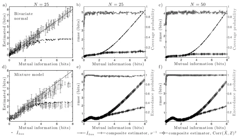
Fig. 1. Bootstrap confidence intervals of the lower boundslog(ν−1/2)can substantially improve inference about mutual information through use of a composite estimator. Simulation results are shown for the bivariate normal (a–c), and for a mixture model incorporating the same linear regression model but with a mixture of normals distribution for X (d–f). N is the number of i.i.d. observations. a) and d): for N = 25, the BCa, nominally90% confidence intervals for our lower bounds in Eqs.6 and 9resp., together with thek-nearest neighbour estimates, Iˆknn, with k= 3. (Analogous confidence intervals for the lower bounds based onCorr( ˜X, Z)2 are shown in d) for the mixture model whenI(X;Z)>4bits). Parameter vectors for each model were sampled independently from their parameter spaces. A single data set is generated for each parameter vector in a) and d). Coverage probability (grey crosses, b) and c)) gives frequency with which theBCainterval covers the trueI(X;Z); Exceedance probability (grey crosses, e) and f)) gives frequency with whichI(X;Z)exceeds the lower limit of theBCa interval (nominally>0.9). Root mean square errors (rmse) are plotted forIˆknn (filled circles), and the composite estimators (see text) based onνZ−|1X orν
−1 ˜
X|Z (black crosses) andCorr( ˜X, Z)
2(diamonds). Results based on 500Monte Carlo replications.
normal distribution (under the data generating density,f), hence(X, Z)has a bivariate normal distribution,X= ˜X, and the boundslog(ν−1/2)in Eqs.6and9hold with equality. In the second,Xis specified to be an equally-weighted mixture of 2 normals, and we obtain the pseudo-input X˜ by first transforming to uniformity using the probability integral transform and then transforming to normality. We adopt the second specification because E[ ˜X|Z]becomes non-linear (and sigmoidal), but the true value of I(X;Z) is still known with precision through the use of a Monte Carlo average for h(Z) (see Appendix). Details of the parameterisations of the models used are also given in the Appendix.
Panels a) and d) of Fig. 1 show our BCa confidence intervals for the lower bounds based on Eq. 6 and 9
respectively, together with the point estimatesIˆknn, for independently generated data sets corresponding to different
true values ofI(X;Z)and for sample size N = 25. In [21], the authors recommend in practice to use values of k between 2 and 4. We therefore calculate Iˆknn usingk= 3nearest neighbours (Iˆknn =I(2)(X, Z;k= 3) in [21]).
The poor performance ofIˆknn with this sample size is evident for both models, particularly for mutual information
in excess of 3 bits, where substantial, growing bias and rmse are evident (see Fig. 2 for plots of bias). Higher values of k result in worse bias and rmse of Iˆknn (not shown). The remaining panels of Fig. 1 depict, for sample sizes
N = 25 and N = 50, various properties under repeated sampling: the frequency with which the BCa interval for the lower bound covers [b) and c)] and has a lower limit exceeded by [e) and f)] the true mutual information; the rmse of Iˆknn; and the rmse of our composite estimator, given by the maximum ofIˆknn and the lower limit of the
BCa interval. For both sample sizes, the nonparametric confidence intervals perform well under repeated sampling and provide substantial reductions in bias and rmse when comparing Iˆknn to the composite estimator (see also Fig.
0 2 4 6 8 −6 −5 −4 −3 −2 −1 0 1 N=25
Mut ual infor mat ion ( bit s )
Bi a s (b it s) 0 2 4 6 8 −5 −4 −3 −2 −1 0 1 N=50
Mut ual infor mat ion ( bit s )
Bi a s (b it s) 0 2 4 6 8 −4 −3 −2 −1 0 1 N=100
Mut ual infor mat ion ( bit s )
Bi a s (b it s) 0 2 4 6 8 −6 −5 −4 −3 −2 −1 0
Mut ual infor mat ion ( bit s )
Bi a s (b it s) 0 2 4 6 8 −5 −4 −3 −2 −1 0
Mut ual infor mat ion ( bit s )
Bi a s (b it s) 0 2 4 6 8 −4 −3 −2 −1 0 1
Mut ual infor mat ion ( bit s )
Bi a s (b it s) ˆ
Ik n n c ompos it e e s t imat or , ν−1 c ompos it e e s t imat or , Cor r ( ˜X, Z)2
d) e ) f )
a) b) c )
Mixt ur e mode l Bivar iat e nor mal
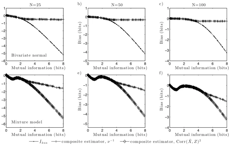
Fig. 2. The lower boundslog(ν−1/2) can substantially reduce bias through use of a composite estimator. The lower bounds based on the Peason correlation do not reduce estimation bias for the mixture model with non-linear conditional mean. Biases are plotted for the k-nearest neighbour estimates, Iˆknn, with k = 3 (filled circles), and for the composite estimators (see text) based onνZ−|1X or ν
−1 ˜
X|Z
(bivariate normal and mixture models respectively; crosses) andCorr(X, Z)2
(diamonds). Parameter vectors for each model were sampled independently from their parameter spaces. Results are shown for the bivariate normal (a–c), and for the mixture model (d–f). N is the number ofi.i.d.observations in each data set. All results based on500Monte Carlo replications.
considerably worse than that based on νX˜|Z, as shown in panels d) to f) of Figs. 1 and 2. The corresponding BCa
intervals lie well below those based on νX˜|Z and have lower limits belowIˆknn in all cases shown in panel d). The
associated composite estimator consequently fails to reduce either the bias or the rmse of estimation.
VII. APPENDIX
A. Additional proofs
Proof: (Lemma 3) Let g(x, z) be the multivariate Gaussian density with the same unconditional first and second moments as f(x, z), and with marginal Gaussian density g(x) = f(x). Thus, Vg[(X, Z)] = Vf[(X, Z)].
We use subscripts to identify the relevant joint density throughout. Notice that
If(X;Z) =Ef log g(X, Z) f(X)g(Z) −Ef logg(X, Z)f(Z) f(X, Z)g(Z) ≥Ef log g(X, Z) f(X)g(Z) ,
where the second expectation of the equality is seen to be non-positive by applying Jensen’s inequality and then integrating first with respect to x. Furthermore,
Ef log g(X, Z) f(X)g(Z) =Eg log g(X, Z) f(X)g(Z) =Ig(X;Z), (13)
because Ef[log{g(·)}] =Eg[log{g(·)}].For example, Ef[log{g(X, Z)}] =Eg[log{g(X, Z)}]because Ef ( X−E[X] Z−E[Z] T Vg[(X, Z)]−1 X−E[X] Z−E[Z] ) = tr ( Vg[(X, Z)]−1Ef " X−E[X] Z−E[Z] X−E[X] Z−E[Z] T#) =d,
since Vg[(X, Z)] = Vf[(X, Z)]. Evaluating Ig(X;Z)=hg(X) +hg(Y) −hg(X, Y) is straightforward since the
marginal and joint densities under g are all Gaussian. We find
Ig(X;Z) = 1 2log det(Vg[X])det(Vg[Z]) det(Vg[(X,Z)]) = 1 2log det(Vf [X])det(Vf [Z]) det(Vf [(X,Z)]) ,
since g andf have identical second moments by construction. The stated results are then obtained by partitioning of the matrix Vf[(X, Z)].
Proof: (Theorem 2). We have that ν(Xn|Zn) = ν( ˘Xn|Zn) → 0. Since ν( ˘Xn|Zn) = E{V[ ˘Xn|Zn]} =
E{(X˘n −E[X˘n|Zn])2}, it follows that X˘n−E[ ˘Xn|Zn] converges to zero in mean square (in L2) and therefore
˘
Xn−E[ ˘Xn|Zn]→pr 0. Consider estimating X˘n based on observation ofZn as follows: the estimator Xˆn(Zn) is
equal to a point in the support ofX˘nwhich minimises the Euclidean distance from E[ ˘Xn|Zn]. Letx∈R,x˘n∈X˘n
and notice that if |x˘n−x|< ∗, then |x˘n−x|< ∗n <|x˘0n−x|, that isx is closer to x˘n than to any other point
˘
xn0 in X˘n. Therefore, if |X˘n−E[ ˘Xn|Zn]|< ∗, E[ ˘Xn|Zn] is closer to X˘n than to any other point in the support,
the estimator Xˆn(Zn) is uniquely defined, and that estimator recoversX˘n without error
ˆ
Xn(Zn) = ˘Xn
. Thus, the probability of estimation error, perror,satisfies
perror=P n ˆ Xn(Zn)6=X˘n o ≤Pn|X˘n−E[ ˘Xn|Zn]| ≥∗ o .
Since X˘n−E[ ˘Xn|Zn]→pr 0, perror must therefore tend to zero as n→ ∞.Fano’s Inequality gives
H(perror) +perrorlog|Xn| ≥H( ˘Xn|Zn) =H(Xn|Zn),
since|X˘n|=|Xn|and the rescaling does not change the conditional entropy. ThereforeH(Xn|Zn)→0asn→ ∞.
Models, parametrisations and algorithms used in the simulation study of Section VI-A
Figures 1 and 2 present simulation results for two data generation mechanisms. In both, Z = βX +ε with ε ∼ N(0, σ2ε) and ε independent of X. The two models, together with the schemes used to generate parameter vectors for the results shown in Figures 1 and 2, are as follows:
1) Bivariate normal model:X ∼N(0, σX2).Model parameters were sampled as follows: i)βuniformly distributed on (1,10); ii) σ2ε = 10θ1 with θ1 uniformly distributed on (−2,2); and iii) σ2X = 10
θ2 with θ
2 uniformly distributed on (−2,2).
2) Mixture model: X is an equally-weighted mixture of 2 normal distributions, that is fX(x) =
1 2N(µ1, σ 2 1) + 1 2N(µ2, σ 2
2). Model parameters were sampled as follows: i)β = 10θ1, withθ1uniformly distributed on(−1,1); ii) σε2= 10θ2 with θ2 uniformly distributed on(−2.5,2.5). We set µ1=−µ2 = 5 and σ12=σ22 = 25/4. The mixture model allows precise evaluation ofI(X;Z) =h(Z)−h(Z|X) via Monte Carlo sampling. We have h(Z|X) = 12log(2πeσε2). Note that the marginal density f(Z) is also an equally-weighted mixture of 2 normals which we can express in closed form. Hence, we can also estimate h(Z) = −E[logf(Z)] as the Monte Carlo average of logf(Zm) where Zm (m= 1, ..., M) is a draw from the mixture model. For our numerical calculations
we set M = 105, and monitored convergence of the Monte Carlo average.
Computations were implemented in R (version 2.12.2). The non-parametric estimation ofE[ ˜X|Z]was performed using the ‘smooth.spline’ function (an implementation of smoothing splines [33]) with the number of knots set to 10; the smoothing parameter was chosen using cross-validation on the original dataset; all other parameters were set to their default values. 90% BCa confidence intervals were calculated from B = 2000 bootstrap replications (using the ‘boot’ package). For the k-nearest neighbour estimation of mutual information [21] we used the authors’ ‘MIxnyn’ function within their MILCA suite (available at http://www.klab.caltech.edu/∼kraskov/MILCA/).
REFERENCES [1] Linfoot, E. H. (1957)Information and Control1, 85–89.
[2] Joe, H. (1989)Journal of the American Statistical Association84, 157.
[3] Brillinger, D. and Guha, A. (2007)Journal of Statistical Planning and Inference137, 1076–1084. [4] Reshef, D. N., Reshef, Y. A., Finucane, H. K., and Grossman, S. R. et al. (2011)Science334, 1518–1524. [5] Shannon, C. E. (1948)Bell System Technical Journal27, 379–423.
[6] Brennan, M. D., Cheong, R., and Levchenko, A. (2012)Science338, 334–5.
[7] Rieke, F., Warland, D., de Ruyter vanSteveninck, R., and Bialek, W. (1999) Spikes: Exploring the Neural Code, MIT Press. [8] Cheong, R., Rhee, A., Wang, C. J., Nemenman, I., and Levchenko, A. (2011)Science334, 354–358.
[9] Bowsher, C. G. and Swain, P. S. (2012)Proceedings of the National Academy of Sciences USA109, E1320–8. [10] Bowsher, C. G., Voliotis, M., and Swain, P. S. (2013)PLoS Computational Biology9, e1002965.
[11] Panzeri, S., Senatore, R., Montemurro, M. A., and Rasmus, S. et al. (2012)Journal of Neurophysiology98, 1064–1072. [12] Prelov, V. and Verd´u, S. (2004)IEEE Transactions on Information Theory50, 1567–1580.
[13] Guo, D., Shamai, S., and Verd´u, S. (2005)IEEE Transactions on Information Theory51, 1261–1282. [14] Guo, D., Shamai, S., and Verd´u, S. (2008)IEEE Transactions on Information Theory54, 1837–1849.
[15] Cover, T. M. and Thomas, J. A. (2006) Elements of Information Theory, John Wiley & Sons Inc., second edition. [16] R´enyi, A. (1959)Acta Mathematica Academiae Scientiarum Hungarica 10, 441–451.
[17] Bernardo, J. M. (1979)The Annals of Statistics7, 686–690.
[18] Bernardo, J. M. and Smith, A. F. M. (2000) Bayesian Theory, John Wiley & Sons Inc.
[19] Dawid, A. P. (2010) Seeing and doing: The Pearlian synthesis. In: Dechter, R., Geffner H., and Halpern J. Y. eds.Heuristics, probability and causality: A tribute to Judea Pearl: College Publications, 309–325.
[20] Mitra, P. P. and Stark, J. B. (2001) Nature411, 1027–30.
[21] Kraskov, A., St¨ogbauer, H., and Grassberger, P. (2004)Phys Rev E69, 1–16. [22] Berger, T. (1971) Rate-Distortion Theory, Prentice Hall.
[23] Gebelein, H. (1941)Zeitschrift f¨ur angew21, 364–379.
[24] Rieke, F., D., W., and Bialek, W. (1993)Europhysics Letters22, 151–156.
[25] Cover, T. M. and Thomas, J. A. (1988) SIAM Journal on Matrix Analysis and Applications9, 384–392. [26] Rosenblatt, M. (1952)The Annals of Mathematical Statistics23, 470–472.
[27] Bowsher, C. G. (2010)The Annals of Statistics38, 2242–2281.
[28] Grima, R. (2010)The Journal of Chemical Physics133, 035101–035101. [29] Thomas, P., Matuschek, H., and Grima, R. (2012)PloS One7, e38518. [30] Friedman, J. H. (1991)The Annals of Statistics19, pp. 1–67.
[31] Bickel, P. J. and Levina, E. (2008) The Annals of Statistics36, pp. 199–227.
[32] Efron, B. and Tibshirani, R. J. (1994) An Introduction to the Bootstrap, Chapman & Hall/CRC.