Bayesian regression for network data

OpenBU http://open.bu.edu

Theses & Dissertations Boston University Theses & Dissertations

2019

Bayesian regression for network

data

https://hdl.handle.net/2144/39324 Boston University

GRADUATE SCHOOL OF ARTS AND SCIENCES

Dissertation

BAYESIAN REGRESSION FOR NETWORK DATA

by

ELIZABETH M.L. UPTON

B.S., University of New Hampshire, 2007

M.Ed., Harvard Graduate School of Education, 2011

M.A., Boston University 2016

Submitted in partial fulfillment of the

requirements for the degree of

Doctor of Philosophy

2019

First Reader

Luis E. Carvalho, PhD

Associate Professor of Mathematics and Statistics

Second Reader

Eric D. Kolaczyk

Professor of Mathematics and Statistics

Third Reader

Daniel L. Sussman

Acknowledgments

Thank you to those in my network who have played a role in my academic development over the past five years. Luis: You are an amazing advisor. You inspire me to learn more and have given me confidence in my own abilities. Your intellectual generosity is unparalleled. Ted: No words can express how appreciative I am of your unconditional support, love, encouragement, and strength. You are my rock. Eleanor: Thank you for reminding me of what is important in life. Always remember “that you are valuable and powerful and deserving of every chance and opportunity in the world.”

ELIZABETH M.L. UPTON

Boston University, Graduate School of Arts and Sciences, 2019

Major Professor: Luis E. Carvalho, PhD

Associate Professor of Mathematics and Statistics

ABSTRACT

The research contained in this dissertation extends modeling methods for network data. Networks are widely used, across a number of disciplines, to represent objects and their interconnectedness. The prevalence of this data structure outlines just one of our motivations for developing novel modeling methods and computational tools that improve our understanding of network-indexed data.

We first consider the problem of statistical inference and prediction for processes defined on networks. We assume that the network of interest is known, and we would like to learn more about an attribute associated with its vertices. Drawing on ideas from functional data analysis, our proposed model consists of node indexed predictors and a basis expansion of their coefficients, allowing the coefficients to vary over the network. We employ a regularization procedure, cast as a prior distribution on the regression coefficients in a Bayesian setup, so that predicted responses vary smoothly according to the topology of the network. We present a novel variable selection technique, introduce efficient expectation-maximization fitting algorithms and Markov Chain Monte Carlo sampling schemes, and provide computationally-friendly methods for eliciting hyper-prior parameters.

Turning to an application, we study occurrences of residential burglary in Boston, v

rates appear to vary sharply across regions or hot zones in the city, we construct a hierarchical model that addresses these issues and gives insight into the spatial patterns and dynamics of residential burglary in Boston.

Finally, with the goal of exploring the relationship between a set of predictor variables and a vertex-pair indexed response, we introduce a flexible approach to modeling network ties. Through a generalized linear model framework, we are able to model weighted and binary edges while investigating a variety of effects or features commonly found in networks. We present algorithms and data representations that allow for efficient inference, and we illustrate and evaluate the benefits of our work on both simulated and real-world networks.

1 Introduction 1

2 Modeling Vertex Attributes 5

2.1 The Graph Laplacian . . . 6

2.2 A Single-Intercept Model . . . 8

2.3 Literature Review . . . 10

2.4 Extending the Single-Intercept Model . . . 13

2.5 Prior Elicitation . . . 14

2.5.1 Controlling Basis Rank Expansions . . . 15

2.5.2 Sequential Centroid Estimator . . . 17

2.5.3 Selecting λ and V0 . . . 19

2.6 Model Inference . . . 20

3 A Case Study: Modeling Occurrences of Residential Burglary 23 3.1 The Data . . . 23

3.2 Extending Model (2.4.2) . . . 26

3.3 Prior Specification and Model Inference . . . 27

3.3.1 Eliciting weights . . . 28

3.3.2 Basis ranks, V0, λω, and λθ . . . 29

3.3.3 Estimating β and γ . . . 30

3.4 Results and Discussion . . . 37

3.5 Simulation Study . . . 41

3.6 Concluding Remarks . . . 43

4.1 From GLM to GGLM . . . 49

4.1.1 Vertex Pair Attributes . . . 51

4.1.2 Calculating the Sufficient Statistics . . . 51

4.1.3 Covariate Class Composition, CCC . . . 55

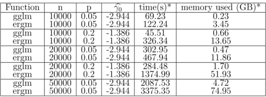
4.2 Additional Extensions . . . 57 4.3 Applications . . . 58 4.3.1 Binary Networks . . . 58 4.3.2 Weighted Networks . . . 63 4.4 Concluding Remarks . . . 64 References 65 Curriculum Vitae 71 viii

4.1 GGLM performance summary . . . 59

0·1 A support network . . . iv 2·1 A toy network . . . 7 3·1 Residential burglary occurrence counts (left) and average wealth

esti-mate (right) for intersections in the network of Boston, MA. . . 24 3·2 Inverse relationship of similarity and distance used to define weights,wij . 28

3·3 Choosingτ based on a threshold of 0.8. . . 30 3·4 Posterior distribution of coefficients with the mean sample value (dashed

line) and the EM-MAP estimates (solid line). . . 37 3·5 Predicted versus actual crime counts for the 13,307 intersections in

Boston, colored by neighborhood. . . 38 3·6 Deviance residuals with hot zone probabilities indicated by grayscale 39 3·7 Left: the value of πv, indicating probability of hot zone (compared to

background rate). Right: wealth effect for each intersection. . . 40 3·8 We compare the relative error from four models for intersections in

each hot zone (HZ) and those intersections not in a hot zone (BG). . 42 4·1 A graph and its corresponding CCC graph (top) and the alternative

ways of representing the data (bottom). In the CCC graph, node weights andyi values are labeled. . . 57

4·2 Random graph generated with a given degree sequence . . . 60

entiated by node color, n = 1000 . . . 61 4·4 CCC graph of Amazon co-purchasing network (loops removed) . . . . 62 4·5 Results of Amazon analysis: 10 product category coefficients and their

standard errors. . . 62

BPD . . . Boston Police Department CCC . . . Covariate Class Composition CP . . . Core-Periphery

CPU . . . Central Processing Unit

CRAN . . . Comprehensive R Archive Network ECM . . . Expectation/Conditional Maximization EM . . . Expectation Maximization

ERGM . . . Exponential Random Graph Model GLM . . . Generalized Linear Model

GGLM . . . Graph Generalized Linear Model IRLS . . . Iteratively Reweighted Least Squares LOOP . . . Leave One Out Proxy

MAP . . . Maximum a Posteriori MCMC . . . Markov Chain Monte Carlo

MALA . . . Metropolis Adjusted Langevin Algorithm

MMALA . . . Manifold Metropolis Adjusted Langevin Algorithm PRESS . . . Predicted Residual Error Sum of Squares

SCC . . . Boston University’s Shared Computing Cluster

Introduction

Advances in data collection have led to the increased presence and availability of network-indexed data. Networks are found in a number of diverse fields including the social sciences, technology, and biology, and allow us to represent complex sys-tems more simply. The term network refers to a collection of elements and their interrelations. We refer to the elements as nodes or vertices, and the relationships we denote as edges. For example, in a friendship network, nodes may correspond to people and edges to friendships; in a gene regulatory network, proteins act as nodes and protein-protein interactions constitute edges; in an airline transportation network, airports may act as nodes and flight paths as edges. These examples illus-trate the universality of networks as powerful tools to represent connected items in a range of disciplinary fields. My dissertation centers on developing novel modeling methods and computational advancements that improve our understanding of this progressively more prevalent data structure. Specifically, my work is motivated by the following two goals: (1) to understand or explain a vertex attribute of interest in a manner that utilizes information from both the network’s structure and pertinent covariates and (2) to offer a logical and flexible framework to model edges or edge responses that can capture basic network properties while retaining computational feasibility.

Mathematically, we represent a network as a weighted graph G = (V, E, w) with

vertex set V, edge set E,and positive weights w, that is, wij >0 whenever (i, j)∈E

for all i, j ∈ V and wij = 0 otherwise. In line with the previously stated goals, we

develop two flexible classes of models, both presented in the framework of Bayesian generalized linear models (GLMs). We have as follows:

Yv|β,γ ind ∼ Fg−1 x>_vβ(v)+z_v>γ β ind∼ N(0,ΩGw) (1.1) Yuv|β, θuv = 1 ind ∼ Fg−1 h(xu,xv) > β θuv|γ ind ∼ Bern logit−1 hL(xu,xv) > γ (1.2)

where Fbelongs to an exponential family and g is a link function, e.g. the canonical link.

In (1.1) the weighted graph under consideration, Gw, is fully known and our

inter-est lies in better understanding a vertex attribute, Yv. Classical regression methods

are not immediately applicable to this setting, as we desire a model that will utilize information from both the network’s structure and node-indexed covariates to explain the response. That is, we want to leverage information found in the connectivity and vertex similarity of the network to describe the dependent variable. We accomplish this by allowing components of the linear predictor, the coefficients β corresponding to node-indexed covariates xv, to vary over the network. We propose a prior on these

varying effects that is informed by the graph and enforces smoothness on the coef-ficients across the network. This construction allows different effects for each node in the network while imposing that similar vertices have similar effects. Effects that are constant across the network are represented in (1.1) by γ with corresponding predictors zv.

construction and interpretable results present a clear picture of how factors con-tributing to the vertex attribute of interest vary across the network. That is, we have developed a model specific to networks, utilizing ideas from functional data analysis, that allow us to incorporate network information in the model’s construction while retaining the flexibility and interpretability of Bayesian GLMs. Chapter 2 of this dissertation provides the details of model (1.1) including novel variable selection techniques, expectation-maximization (EM) fitting algorithms, and a Markov Chain Monte Carlo (MCMC) sampling routine that provides the posterior distribution of the coefficients. The flexible construction of our model makes it applicable to modeling a variety of network data sets where the network structure plays a role in explain-ing a vertex-indexed variable. In chapter 3, we explore one significant application: modeling occurrences of residential burglary.

We first note that analyses of occurrences of residential burglary in urban areas show that crime rates are not spatially homogeneous: rates vary across regions in the city resulting in some neighborhoods being considered far more susceptible to crime than others. Motivated by the importance of understanding these spatial patterns, we consider model (1.1) in the context of modeling occurrences of burglary defined on the network of city streets in Boston, Massachusetts. We introduce a network-indexed latent binary variable that differentiates between two crime rates (a background crime rate and a “hot zone” crime rate) and show that incorporating this variable along with network structure leads to a more representative and informative model.

In (1.2) our interest is in performing inference on graph structure or edge attributes in an undirected network. The functionshandhLwith node specific inputsxu andxv

encode vertex-pair covariate information used to infer an edge-indexed response. The hierarchical structure of our model allows for a zero-inflated formulation where the process behind the existence (or non existence) of an edge may be different than that

generating the edge attribute we are interested in modeling. Through this flexible regression framework, we are able to investigate a variety of effects that may shape a network, such as degree heterogeneity and clustering. Furthermore, the response in model (1.2) is not constrained to the binomial or Poisson case as is common in many network regression formulations.

We explicitly note that our model specification in (1.2) assumes dyadic indepen-dence; edges and their values are independent given the model parameters. While this limitation is not present in the more general exponential random graph models (ERGMs), model (1.2) benefits from exact and relatively straightforward calculation of the maximum likelihood parameter estimates. Given this simplification, we de-sign fitting algorithms and data representations that allow for efficient inference on large and dense networks where similar analyses in the ERGM framework are not feasible. These graph generalized linear model (GGLM) procedures are introduced and detailed in chapter 4. We also illustrate and evaluate the benefits of our work on both simulated and real-world networks. Recognizing the import of making the GGLM procedures available to the statistical community, we outline the capabilities and syntax of our corresponding R (R Core Team, 2018) package,gglm.

Modeling Vertex Attributes

Given a network where vertices are connected by weighted edges, we observe vertex-indexed data in the form of vertex attributes. As common in many applications, we distinguish between a response attribute of interest and a set of predictor attributes, and let the edge weights capture a measure of similarity between vertex attributes. Some examples include the infection status of individuals in a friendship network of injection drug users given their drug use habits and other covariates such as age and gender; the political party affiliation of web blog authors in a network of hyper-linked connected blogs given the distribution of post topics and readership ideological inclinations; and the functional classes of proteins in a network of proteprotein in-teractions given gene pathway and other biological information (Leskovec and Krevl, 2014). The edge weights in the network are assumed to indicate vertex affinity and adjacent or close vertices are similar on some characteristic level relevant to the vertex attribute of interest. Our main goal is to model the response attribute using regres-sion, but in a way that explores the topology and vertex similarity information in the network. Furthermore, we want to address effect nonhomogeneity, that is, a situation where the covariate effects are not constant across the network. This is a critical ex-tension in modeling network attributes, as dynamic patterns may exist between the response variable and predictor attributes that depend on the local structure of the network. It is sensible then to adapt the well-known constant coefficients regression

model to a functional or varying coefficients formulation (Hastie and Tibshirani, 1993; Ramsay and Silverman, 2005).

The remainder of this chapter is organized as follows. First, we define the graph Laplacian and comment on its properties that are relevant to our discussion. Then, we simplify the regression problem by examining an “intercept-only” model, that is, a model informed only by the vertex similarly in the network. This leads to a literature review describing current research in this area. We then extend our intercept-only model to include pertinent covariates; here, our methodology is novel and results in complete specification of model (1.1) presented in the introduction. Lastly, we discuss necessary extensions such as hyper-prior parameter selection, a new covariate selection method, and efficient model fitting techniques.

2.1

The Graph Laplacian

Consider a weighted graph, Gw, with Nv vertices. The weighted graph Laplacian,

Lw, is a symmetric matrix defined as Lw = Dw −W with W = [wij], the weighted

adjacency matrix, andDw = Diagi∈V{

P

j∈V wij}, a diagonal matrix with the weighted

degrees. The graph Laplacian is called such due to it being the finite-difference analog of the continuous Laplacian operator ∆ = _∂x∂22

1 + ∂2 ∂x2 2 +· · ·+ ∂2 ∂x2 m. In a quadratic form, first noting we can write Lw = P_e∈ELwe, where Lwe is the graph Laplacian of the graph consisting of one edge and Nv vertices, we have for any real valued vectorx,

x>Lwx=x> X e∈E Lwe x=X e∈E x>Lwex= X (i,j)∈E wij(xi−xj)2. (2.1.1)

Thus, we see that the Laplacian can be used to quantify how much x varies locally over the graph (Smola and Kondor, 2003). It follows directly from (2.1.1) that Lw

is positive semi-definite with eigenvalues, 0 = λ1 ≤ λ2 ≤ · · · ≤ λn and an

eigen-decompositionLw = ΦΞΦT.The eigenvalues and eigenvectors of the graph Laplacian

can be used to describe properties of the graph, for example, the number of connected components. The eigenvectors correspond to functions partitioning the graph into similar components and are commonly used in conjunction with K-means algorithms to perform spectral clustering on the nodes. See Von Luxburg (2007) for further details.

A useful factorization of the graph Laplacian is Lw = M>M, where M is the

weighted oriented incidence matrix. The incidence matrix is an |E| ×Nv matrix

where, for e= (i, j)∈E, Me,vi =

√

wij, Me,vj =−

√

wij and Me,vk = 0 for all k ∈V,

k 6=i and k 6=j. As an example, for the network pictured in figure 2.1, we have,

Figure 2·1: A toy network

M =     √ 10 −√10 0 0 0 √5 −√5 0 0 √4 0 −√4 0 0 √3 −√3     and Lw =     10 −10 0 0 −10 19 −5 −4 0 −5 8 −3 0 −4 −3 7     .

For completeness, we include the proof of the factorization of the graph Laplacian.

Differ-ent versions of this proof exist; for example, see Godsil and Royle (2013, Section 8.3). We have [M>M]ij = the inner product of the ith andjth columns ofM.Splitting this

• i=j : [M>M]ij = X e∈E [Me,vi] 2 _{= deg} w(i) • i6=j and (i, j)∈/ E : [M>M]ij = X e∈E [Me,vi][Me,vj] = 0

as every edge is non incident to either vi orvj

• i6=j and (i, j)∈E : [M>M]ij = X e∈E [Me,vi][Me,vj] = X e=(i,j) [Me,vi][Me,vj] =−wij.

We now make use of the weighted graph Laplacian and corresponding incidence matrix in our regression formulation.

2.2

A Single-Intercept Model

Let us assume for the moment that we have a single, vertex-indexed, intercept model,

Yv|β

ind

∼ F[g−1_{(β(v))] where F belongs to an exponential family and g is a link} func-tion. Given that each vertex has its own intercept value, the model hasNv parameters

and will clearly over fit; rather than summarize the data, the model merely interpo-lates the data and is uninformative in this setting. We thus impose smoothness on β through a prior. Given that the fundamental principle of Bayesian statistics is to incorporate prior knowledge when fitting model parameters, it is natural to exploit in-formation found in the structure of the given graph to inform our model. Specifically, we use the weighted graph Laplacian and a roughness penalty λ > 0 for the prior

formulation: β ∼ N(0, λ−1_L

w−). Note that Lw1|V| = 0 and so Lw is rank deficient,

requiring the use of the generalized inverse L−_w when defining the prior.

Now, using Bayes’ rule we have _P(β|Y) ∝ _P(Y|β)_P(β) and we can find the posterior distribution ofβ using a sampling algorithm. Alternatively, we can find the maximum a posteriori (MAP) estimate βb for β as

b β= argmax β n P(Y|β)P(β) o = argmax β n log _P(Y|β)_P(β)o = argmax β n `(β;Y)− λ 2β >_M> wMwβ o = arg min β n D(Y, g−1(β)) +λβ>M_w>Mwβ o

where ` is the model log-likelihood and D is the model deviance, and Mw is the

weighted oriented incidence matrix. In the GLM setting, the deviance is formed from the logarithm of the ratio of likelihoods, and is used to measure goodness of fit (specifically, the discrepancy of a model’s fit is proportional to twice the difference between the maximum log likelihood achievable and that obtained by the model under consideration (McCullagh and Nelder, 1989, Section 2.3)).

Our choice of Mw in the prior formulation exploits the identities outlined in 2.1

to leverage the network topology and edge weights for regularization. Expanding the log prior using (2.1.1), we have

β>M_w>Mwβ=β>Lwβ=

X

(i,j)∈E

wij(β(i)−β(j))2, (2.2.1)

that is, the term penalizes the weighted sum of squares of the difference of the co-efficients between adjacent vertices in the network where the weights, wij capture

a measure of similarity between connected vertices (Kolaczyk, 2009, Section 2.1.3). Thus, we are seeking estimates of β(v) that balance representativeness with respect to our observed dataY andX in the likelihood with smoothness with respect to the network topology in the prior. The parameterλ is used to calibrate this balance.

The network effects β can be conveniently represented using a basis expansion with respect to the eigenvectors of Lw, a common approach in functional data

anal-ysis (Ramsay and Silverman, 2005). More specifically, we can take τ eigenvectors to represent β asβ = Φ1:τθ, where Φ1:τ contains the firstτ eigenvectors of Lw, ordered

by the eigenvalues ξ1 <· · · < ξτ. Using this formulation, the log prior becomes (up

to a constant) −λ 2β > Lwβ =− λ 2θ > Φ>_1:τΦΞΦ>Φ1:τθ=− λ 2θ > Diag_i=1,...,τ{ξi}θ,

which is equivalent to θ∼N(0, λ−1_Diag

i=1,...,τ{ξ

−1

i }). This results in the MAP

b θ = arg min θ n D Y, g−1(Φ1:τθ) +λθ>Diag_i=1,...,τ{ξi}θ o . (2.2.2)

Thus, we can use our GLM machinery to findθb,and then perform matrix

multiplica-tion using τ eigenvectors of the graph Laplacian to back out the estimate of β. The result is a vertex-indexed intercept that varies smoothly over the network.

2.3

Literature Review

Similar approaches have been followed before in the context of kernel regression on graphs (Smola and Kondor, 2003; Belkin et al., 2004). Kernel based algorithms are commonly used to operate on discrete input spaces (e.g. Kolaczyk, 2009, Section 8.4) where the kernel, K, acts as a function that quantifies the similarity between two

inputs. The “predictor variables” are then dervied from the kernel. K must satisfy two mathematical requirements to act as a kernel: it must be symmetric, and positive semi-definite (Kondor and Lafferty, 2002). Naturally then, the graph Laplacian is often used in the formation of kernels when the goal is to approximate data on a graph; see Smola and Kondor (2003) for a number of examples of kernels defined via the Laplacian. These kernel methods interpret the log prior given in 2.1.1 as a penalty for a (log) Gaussian or Bernoulli likelihood. Similarly, Belkin et al. (2004) consider the problem of labeling a partially labeled graph through regularization algorithms using a smoothing matrix,S,such as the Laplacian, and discuss theoretical guarantees for the generalization error of the presented regularization framework based on the second smallest eigenvalue of S.

While these model formulations capture information in the network topology, they do not allow us to easily incorporate pertinent covariates. Kernel methods have been extended to include information from multiple kernel functions, each arising from a different data source. See for example Lanckriet et al. (2004). In this case, different kernel functions are used to capture different notions of similarity, and the problem is redefined as determining an optimal vector of weights, µ, used to merge the various kernels. That is, given a set of kernels,_K={K1, K2, . . . , Km},they define

a combination kernel as K = m X i=1 µiKi

where each µi ≥ 0. This is a convex optimization problem which the authors solve

using semidefinite programming (Lanckriet et al., 2004). However, these nonpara-metric methods often lack interpretability beyond analyzing the µi values and suffer

from computational issues.

covari-ates (Li and Li, 2008). The proposed procedure involves a smoothness penalty on the coefficients derived from the Laplacian, however, in this particular application it is the predictor variables that represent the vertices in a graph, and the presence or absence of an edge identifies correlated features. The question of interest revolves around identifying grouping effects for predictors that are linked in the network. While the machinery employed is similar to that previously discussed, the question of interest is essentially different.

With the increased popularity and availability of network data, developing a framework for regression models specific to network indexed data has become a focus of recent research. Li et al. (2016) discuss network prediction models that incorpo-rate network cohesion, the idea that linked nodes act similarly, and node covariates. Their model includes individual node effects instead of a single intercept, and they introduce a cohesion penalty based on the Laplacian. They develop the theoretical properties of their estimator and demonstrate its advantage over regressions that ig-nore network information. Similarly to Li et al., our full model, specified in (1.1) focuses on interpretability and generalization; learning about the network and the vertex attribute of interest by examining the covariate values and introducing a flexi-ble framework adaptaflexi-ble to a variety of GLM settings. However, our method differs in that Li et al. assume the effect of the covariates is the same across the network, while we address the issue of non-homogeneity by representing the coefficients using a basis expansion with respects to the eigenvectors of the Laplacian. That is, our proposed model allows for interpretation of how a covariate’s influence on the attribute process of interest changes across the network. We now outline this novel methodology.

2.4

Extending the Single-Intercept Model

We want our model to include vertex indexed covariate information leading to better predictive power and further understanding of the vertex attribute process. That is, given p predictors, we wish to regress the vertex attribute on

ηv =g(E[Yv]) =β0(v) +x1vβ1(v) +· · ·+xpvβp(v).

We perform the same basis expansion described in the intercept model on each coef-ficient, using the firstτj eigenvectors of L, yielding

ηv = p X j=0 xjvβj(v) = p X j=0 xjvφ>τ vθj

that is, withβj(v) = φ>τ vθj whereφτ v is the v-th row in Φ1:τj and we identifyx0v = 1 for the intercept. Note that we can write η=DXθ where

DX = [Φ1:τo Diagv∈V{x1v}Φ1:τ1 · · · Diagv∈V{xpv}Φ1:τp]

andθ = [θ0 θ1 · · · θp]. We choose to smooth the linear predictor η over the network,

resulting in predictions for the vertex attribute that vary smoothly over the topology of G. This new, more general specification extends the posterior estimate in (2.2.2) to accommodate the roughness penalty λη>Lwη=λθ>DX>LwDXθ:

b θ= argmin θ n D Y, g−1(DXθ) +λθ>D>_XLwDXθ o (2.4.1)

and results in the priorθ ∼N(0, λ−1_(D>

XLwDX) −

) for the basis expansion coefficients. Putting the pieces together in the Bayesian GLM framework we have

Yv|θ ind ∼ Fhg−1 DX(v)>θ i θind∼ N 0, λ−1(D>_XLwDX) − (2.4.2) in accordance with (1.1).

2.5

Prior Elicitation

Fitting the proposed model to data requires eliciting hyper-prior parameters. In particular, we need to select:

Basis ranks τj. The cardinalities of the network basis expansions control how

long-range, global network effects in DX affect the prior precision for θ. To elicit

these ranks, we introduce a modified spike-and-slab prior (George and McCul-loch, 1993) and corresponding expectation/conditional maximization (ECM) algorithm (Meng and Rubin, 1993) to perform variable selection. In the typical spike-and-slab variable selection routine withppredictors, 2p _{models composed}

of all possible subsets of the predictors are explored. However, our methodol-ogy allows us to traverse the eigenvectors of the Laplacian sequentially, for each

j-predictor, to determine τj.

Roughness penalty λ. This precision scale parameter controls the amount of reg-ularization or smoothing of the β coefficients. We elicit this parameter, along with a hyper-parameter controlling the variance between spike and slab when selecting the ranks τj, based on a criterion to minimize prediction error.

2.5.1 Controlling Basis Rank Expansions

Given there are Nv Laplacian eigenvectors and we perform a basis expansion on

each coefficient in our model, it is likely we will find ourselves in a high-dimensional setting. While we would like τj to be large enough so that the combination of the

τj eigenvectors reflects characteristics of our attribute process, we wish to keep the

computational expense of our model in check (Ramsay and Silverman, 2005). To this end, we modify the model previously presented, 2.4.2 in section 2.4, by setting a hyper-prior on the basis ranks τj and performing Bayesian variable selection on the

basis coefficients. More specifically, we adopt the prior structure,

θj|τj ind ∼ N0, λ−1M_τ1/2 j (D > XjLwDXj) − M_τ1/2 j (2.5.1)

where, with K ≤ |V| the maximum basis rank, I the indicator function, and DXj = Diag{Xj}Φ1:K, we haveMτj = Diagi=1,...,K{I(i > τj)V0+I(i≤τj)}. Here 0< V0 1 is a small value distinguishing the separation between the variance of the spike and slab components. That is, the prior distribution of θj given τj is a mixture of two

normal distributions centered at zero, one with small variance (the spike), and one with large variance (the slab).

For the hyper-prior we set

P(τj) =                1−α0, τj = 0 α0(1−α1), τj = 1 α0α1ρτj−1/ PK k=2ρk −1_{, τ} j = 2, . . . , K. (2.5.2)

Given this distribution, hyper-parameters α0 =P(τj >0) and α1 =P(τj >1|τj >0)

expansion, respectively. Thus, parameters α0 and α1 can be elicited directly based on expert opinion of the odds of a predictor being included in the model and, if that is the case, its effect varying over the network. Since ρ=_P(τj =i)/P(τj =i−1) for

i = 2, . . . , K, this parameter controls, in effect, the cardinality of the expansion. To specify ρ, we recommend first finding a representative value for ¯τ =_E[τj] and then,

given α0 and α1, solving for ρ. That is, we need to solve, according to (2.5.2),

E[τj] =α0(1−α1) +α0α1 PK k=2kρ k−1 PK k=2ρk−1 =α0(1−α1) +α0α1 1 + PK−1 k=1 kρ k PK−1 k=1 ρk ! = ¯τ . Let S(ρ) =. PK−1 k=1 kρ

k_{. Recognizing a variant of the geometric series we have (1−}

ρ)S(ρ) =PK−1 k=1 ρ k_−(K−1)ρK _and PK−1 k=1 ρ k_=ρ(1−ρK−1_{)/(1−ρ), thus,} ¯ τ −α0 α0α1 = S(ρ) PK−1 k=1 ρk = 1 1−ρ − (K−1)ρK−1 1−ρK−1 .

The solution, constrained to ρ > 0, can then be solved numerically using standard procedures such as Newton’s method.

A reasonable choice for ¯τ is the smallest value such that Pτ¯

k=2ξ −1 k / PK k=2ξ −1 k is

bounded by a large value close to 1, e.g. 0.9, similar to the usual variance explained or scree plot methods used to retain components in principal component analysis. We discuss specifying the spike-and-slab variance ratio V0 in Section 2.5.3.

Now, in the spirit of Roˇckov´a and George (2014), we employ an ECM algorithm for model (2.5.1) where we cycle over eachj-th predictor to infer conditional posterior modes for θj with τj as latent variables. That is, we optimize the expected log joint

distribution:

by alternating between the E and CM steps. For the E-step we compute, at the t-th iteration, ν_i(t) =_E[I(i > τ)] = i−1 X l=1 P(τ =l|Y,θ(t)) where _P(τ =l|Y,θ(t)) = P(θ (t)_{|τ =l)} P(τ =l) PK l=1P(θ(t)|τ =l)P(τ =l) .

Next we update θ by maximizing (2.5.3), a process that depends on the conditional distribution of Y, F, and the information from the remaining p predictors in the model. We iterate between the E and CM steps until convergence is determined. After convergence, we select τj via sequential centroid estimation (Carvalho and Lawrence,

2008), which tends to be more robust than the usual conditional posterior mode and, in effect, picks the minimum number of eigenvectors such that the cumulative posterior is less than some threshold. This procedure is repeated for each one of the (p+ 1) predictors in turn until τ does not change between consecutive cycles.

2.5.2 Sequential Centroid Estimator

Let us first define an auxiliary variableω(τ) that represents τ (we drop the subscript

j for the remainder of this section) as an indicator vector: ω(τ)i = I(i ≤ τ), for

i= 1, . . . , K. For instance, ω(0) = (0,0, . . . ,0), ω(1) = (1,0, . . . ,0), and so on, with ω(K) =1K. Note the one-to-one correspondence between τ and ω, and thus, while

τ ∈ T =. {0, . . . , K},ω only takes values in Ω=. ∪j∈Tω(j).

Now, given the marginal posteriors _P(τ|Y) or the EM-conditional posteriors

ac-cording to a generalized Hamming gain Gon the ω-map: b τ = argmax. e τ∈T X τ∈T G ω(_eτ),ω(τ)πτ.

When comparing two indicator ranks, the gain function G assigns zero gain to each discrepancy between them, a unit gain to matched zeroes (true negatives) and a gain of

κ >0 to matched ones (true positives). For example, ifK = 7, thenG(ω(3),ω(5)) = 2 + 3κsince there are three matched ones from positions 1 through 3, two mismatches from positions 4 and 5, and two matched zeros from the last two positions, 6 and 7. Thus, G ω(τ1),ω(τ2) =K−max{τ1, τ2}+κmin{τ1, τ2}. Then, b τ = argmax e τ∈T X τ∈T κmin{τ,_eτ} −max{τ,τ_e}πτ = argmax e τ∈T ( X τ≤eτ (κτ −_eτ)πτ + X τ >eτ (κ_eτ−τ)πτ ) = argmax e τ∈T ( X τ≤_eτ ((κ+ 1)τ−_eτ)πτ+ X τ >eτ κ_eτ πτ ) = argmax e τ∈T ( (κ+ 1)X τ≤_eτ τ πτ −eτP(τ ≤eτ|Y) +κeτ 1−P(τ ≤eτ|Y) ) = argmax e τ∈T n (κ+ 1)_Eτ|τ ≤_eτ ,Y+τ_eκ−(κ+ 1)_P(τ ≤_eτ|Y) o ,

that is,_bτ = argmax

e

g(0) = 0; in general, g(j) = (κ+ 1) j X i=0 iπi+j κ−(κ+ 1) j X i=0 πi =κj+ (κ+ 1) j X i=0 (j−i)πi | {z_. } =sj . But since sj =j Pj i=0πi− Pj

i=0iπi, it follows that

sj+1 = (j+ 1)( j X i=0 πi+πj+1)− j X i=0 iπi−(j+ 1)πj+1=sj + j X i=0 πi. Thus, g(j+ 1) =κ(j+ 1)−(κ+ 1)sj+ j X i=0 πi =g(j) +κ−(κ+ 1) j X i=0 πi,

and so g(j+ 1) > g(j) if and only if κ−(κ+ 1)Pj

i=0πi, that is, κ >

Pj

i=0πi/(1−

Pj

i=0πi), whenκexceeds the cumulative odds. Thus, since

Pj i=0πiis non-decreasing, we conclude that b τ = max ( e τ ∈ T : e τ X τ=0 πτ < κ 1 +κ ) ,

so we propose to expand the basis expansion up to when the cumulative posterior exceeds the κ/(1 +κ) threshold.

2.5.3 Selecting λ and V0

Here we use a leave-one-out cross validation PRESS statistic defined on the working responses in the final step of the iteratively reweighted least squares (IRLS) algorithm, the usual computational routine used to fit generalized linear models (McCullagh and

Nelder, 1989, Section 2.5). We call this the LOOP (leave-one-out-proxy) statistic, LOOP =X v∈V (Yv−µb(v),v) 2 V(µ_b(v),v) ≈X v∈V r_v2 1−hv ,

where µ_b(v),v is the mean at v fitted without the v-th observation, V(µb) is the

es-timated variance function for the distribution concerned, r2

v = (Yv −bµv)

2

/V(µ_bv) is

the Pearson residual, and hv is the leverage at v. While a closer approximation is

provided by Williams (1987), our formulation is computationally convenient.

We define V0, the spike and slab variance ratio, jointly with λ. That is, for a particularV0 value, we find the corresponding basis expansions,τ, via the spike-and-slab prior (see section 2.5.1). We use τ to define DX, and then minimize the LOOP

to determine λ. Using this updated λ, we find new values for τ. The process repeats until there is no change in τ and λ between iterations. The procedure is completed for a range of V0 values, and the combination of V0 and λ that minimizes the LOOP (i.e., the prediction errors with respect toY) determines these parameters in the final model. This process can be viewed as an empirical Bayes procedure where we are optimizing the prediction accuracy rather than the likelihood.

2.6

Model Inference

After determining the dimension ofDX and specifying the hyper-prior parameter λθ,

we are in the position to estimate model parameters. To this end, we sample from the posterior distribution of θ using a one-step Riemannian manifold Hamiltonian Monte Carlo proposal, also known as a manifold Metropolis adjusted Langevin algo-rithm (MMALA); see Girolami and Calderhead (2011). Given the target density may be high dimensional, this sampling algorithm can provide efficient convergence and

exploration of the target density in comparison to more commonly used Metropo-lis Hastings schemes such as the IRLS method presented in Gamerman (1997) or the preconditioned MALA (Girolami and Calderhead, 2011). The MMALA proposal mechanism generalizes the MALA, based on a Langevin diffusion, by taking into ac-count the natural geometry of the target density and making transitions proposals that are informed by its local structure. Specifically, the proposal density is a normal distribution, with mean based on the local curvature of the space along the direction of steepest gradient and covariance given by the scaled inverse Fisher information matrix of the posterior. The process, in the general case, is as follows:

1. Set t= 1 and begin with θ =θ(0)_; 2. Sample θ∗ from proposal density, q;

3. Accept with probability, ρ(θ(t−1)_,θ∗_{).If accept,θ}(t)_=θ∗_{; if reject,θ}(t)_=θ(t−1)_; 4. Set t = t + 1 and return to step 2.

Hereq(θ∗|θn, ) =N θ∗|µ(θn, ), 2G−1(θn) where µ(θn, )i =θni + 2 2{G −1 (θn)∇θlog{p(θn)}}i−2 D X j=1 G−1(θn)∂G(θ n₎ ∂θj G−1(θn) _ij+ 2 2 D X j=1 G−1(θn) _ijtr ( G−1(θn)∂G(θ n₎ ∂θj ) ,

is a step parameter, and G is the Fisher information matrix of the posterior distri-bution. Furthermore we have,

ρ(θ(t−1),θ∗) = min 1, π(θ ∗_)q(θ(t−1)_|θ∗₎ π(θ(t−1)_)q(θ∗_|θ(t−1)₎ ,

130 of Girolami and Calderhead (2011) for further details. We also provide examples in section 3.3.3, along with step size and initial value recommendations, for additional reference.

Now that we have defined our model and outlined fitting procedures and guidelines for hyper-prior parameter selection, we turn to a case study.

A Case Study: Modeling Occurrences of

Residential Burglary

Occurrences of residential burglary in urban areas are not spatially homogeneous. Crime rates vary across the city causing some areas to be heavily impacted by crime in comparison to others. Motivated by the importance of understanding these spatial patterns, we apply the statistical model outlined in chapter 2 defined on the network of city streets in Boston, Massachusetts. Our resulting model and interpretations provide valuable insight into the spatial dynamics of residential burglary in the city. This chapter is organized as follows: in section 1, we introduce and describe our data; in section 2 we apply and extend model (2.4.2) to meet the needs of our application; section 3 outlines hyper-prior specification and examines the posterior distribution of fitted coefficients; section 4 continues with a discussion of our results; section 5 describes a simulation study used to assess the performance of our model; and the chapter concludes in section 6 with a summary of our contributions to modeling vertex attributes.

3.1

The Data

We are interested in a specific type of urban crime, residential burglary. Burglary can be legally defined as “the act of breaking and entering a building with the intent to commit a felony” (Garner, 2001). Our network of interest, the street network of

Figure 3·1: Residential burglary occurrence counts (left) and average wealth estimate (right) for intersections in the network of Boston, MA.

Boston, Massachusetts, contains 18,889 streets segments (edges) and 13,308 intersec-tions (vertices) forming an undirected simple graph.

The crime data, maintained by the city of Boston and available to the public (City of Boston, 2016; Open Data, 2016) consists of crime incident reports provided by the Boston Police Department (BPD) to document the initial details surrounding an incident to which BPD officers respond. The complete data set contains fields categorizing the type of incident, as well as when and where it occurred. We focus on the 7,012 reported instances of residential burglary that occurred between July 2012 and October 2015. We pooled the data over time and mapped each occurrence to its closest intersection. Figure 3·1 pictures each street intersection in the city colored to indicate the value of our attribute of interest, counts of residential burglary occurrences. The attribute covariates gathered and included in our final model are:

Distance from each intersection to the nearest police station.

Sub-district designation of intersection location (business, residential, or other).

Gross tax amount for each parcel in the city of Boston in 2015. To convert gross tax

into a vertex indexed covariate, we construct a buffer around each intersection and then aggregate the fractions of gross tax from each parcel in proportion to the parcel area covered by the buffer.

Predictor attributes analyzed but not present in our final model include population measures, a majority-minority ethnicity composition indicator, neighborhood clas-sifications, and an English language proficiency indicator. Our choice of analyzing the aforementioned covariates was driven by available data and established crime theory (Bernasco and Block, 2009). A variable selection process was also used (see section 3.3.2).

A naive approach to modeling crime counts on each intersection would entail identifying a set of predictor attributes describing each intersection and performing count regression, for instance, Poisson or negative binomial regression. That is, if

Yv and xv are the crime occurrence counts and covariate attributes at vertex v, we

could suppose Yv

ind

∼ Po[exp(xT

vβ)]. However, this specification assumes that crime

effects β are constant over the network and thus spatially homogeneous. Empirical evidence suggests otherwise; for example, figure 3·1 displays gross tax information for the city of Boston in 2015. Comparing this attribute to the counts of residential burglary, we see that in some areas of the city higher taxes, indicative of wealth, correspond to larger crime rates, while in other locations lower taxes, identifying poorer neighborhoods, correlate with higher crime rates. Thus, even when including informative covariates, a simple regression cannot adequately explain the variability in burglary occurrences across a city.

Moreover, the existence of crime “hot spots,” areas of concentrated crime counts, is widely acknowledged in crime theory literature (see, e.g., Eck et al., 2005). These zones can be identified visually in figure 3·1; for instance, in the southern region of the northwest peninsula neighborhood, Allston. Many current crime mapping algorithms, including kernel intensity estimation and univariate time series models, focus on iden-tifying these hot spots. A variety of qualitative theories, such as the routine-activity and broken-window theories, aim to describe hot spot propagation (Eck et al., 2005). Yet, interpretative models providing probabilities of hot spot formulation accounting for and explaining heterogeneous effects seem to be lacking.

Our proposed model aims at capturing both gradual variations in crime explained by predictor attributes and abrupt variations attributed to a hot spots. The inter-pretability of the model allows not only an understanding as to what makes certain parts of the city more susceptible to burglary, but identifies how the factors contribut-ing to high crime change across the city. With this information local law enforcement can direct crime prevention efforts to narrowly defined regions of the city and identify area specific interventions to decrease the occurrence rate of residential burglary.

3.2

Extending Model

(2.4.2)

In chapter 2 we introduced a generalized linear model for vertex attributes that allows the coefficients to vary smoothly over the network. For our application of modeling occurrences of residential burglary, we letFbe Poisson andg = log,the canonical link.

Dx is composed of the aforementioned covariates combined with the eigenvectors of

the weighted graph Laplacian of the street network of Boston. The details of the ECM algorithm used to determine the basis rank expansion of the β coefficients presented in section 2.5.1 are further developed in 3.3.

To address the issue of crime hot spots, we add an additional level of flexibility to the model, allowing it to detect abrupt changes in the vertex attribute over the topology of the graph. That is, we introduce a network-indexed latent binary variable Z,

Zv|γ

ind

∼ Bernhlogit−1 U_v>γ(v)i, (3.2.1) where a set of predictor attributes U and network-smoothed effects γ determine the odds of v belonging to a normal or changed state. In our particular context, this variable allows us to discriminate between two crime rates: if Zv = 0 the vertex is

considered to be located in a crime hot zone where the crime rate is described by the predictors included in our model; ifZv = 1 the vertex lies in an area of the city with

a flat crime rate, a “background” rate ζ. The latent effects γ assume the same basis expansion as previously described in 2.4 for the main effectsβ, that is,γj(v) =φ>τ vωj

and so the linear effects are U_v>γ(v)=DU(v) >

ω, withDU defined similarly toDX.

All together, our final model takes the form

Yv|ζ,θ, Zv ind ∼ Pohexp Zvζ+ (1−Zv)(DX(v) > θ)i Zv|ω ind ∼ Bernhlogit−1 DU(v) > ωi θind∼ N0, λ_θ−1(D>_XLwDX) − ωind∼ N 0, λ−_ω1(D>_ULwDU) − . (3.2.2)

3.3

Prior Specification and Model Inference

Fitting the proposed model to our crime data requires the preliminary step of eliciting hyper-prior parameters. In addition toτj (the basis ranks),λθ (the roughness penalty

on the main level), andV0 (the spike and slab variance ratio) discussed in 2.5, we also need to select the Laplacian weights, w, and the roughness penalty λω affecting the

amount of regularization or smoothing of the γ coefficients. 3.3.1 Eliciting weights 0.0 0.2 0.4 0.6 0.8 1.0 0.0 0.2 0.4 0.6 0.8 1.0

Creating a Weighted Adjacency Matrix based on Similarity

Distance

Similar

ity

Figure 3·2: Inverse relationship of similar-ity and distance used to define weights, wij

Our model is constructed on the premise that adjacent or similar vertices in the network are somehow related in terms of crime counts. The notion of smoothing our linear predictor over the network de-pends on how we define this similarity through edge weights,wij in 2.2.1. Given

that the edges in our network are streets, a natural similarity measure between ad-jacent intersections is an inverse of street distance. As the pure reciprocal function relating similarity to distance will tend to infinity as distance tends to zero, caus-ing computational problems, we employ an exponential decay function (Banerjee

et al., 2014) to define weights, wij ∝ exp{−d(i, j)/ψ}. Here, ψ is a range parameter

and we set max{wij} = 1 to avoid identifiability issues with the roughness

penal-ties. We define ψ such that the similarity weight distribution is not too peaked. Specifically, we select ψ such that the median distance maps to 80% similarity (see figure 3·2), resulting in ψ = 0.162. This pragmatic approach allows the model to effectively differentiate between intersections that are close together and far apart, ensuring that the range of distances in the city network corresponds to an appropriate range of weights. We note that allowing this parameter to vary over the network was

explored, but did not significantly improve our model.

3.3.2 Basis ranks, V0, λω, and λθ

Following the discussion in section 2.5.1, for a particular θj, τj, and DXj = [Diag{Xj}Φ1:K] we have: Yv|θ, τ ind ∼ Po exp(DX(v)>θ) andθ|τ ∼N 0,Σ where Σ = λ−1_M1/2 τ (D>_XLwDX) − Mτ1/2 and Mτ = Diagi=1. . . K{I(i > τ)V0+ I(i ≤ τ)}. τ is as defined in (2.5.2) where ρ = 0.92 is found by choosing ¯τ = 12, the smallest value such that P¯τ k=2ξ −1 k / PK k=2ξ −1 k is bounded by 0.95.

The E step is exactly as in section 2.5.1, where ν_i(t) = _E[I(i > τ)]. For the CM step, we set θ(t+1) by maximizing the expected log likelihood given in (2.5.3):

Q(θ;θ(t)) =c−vexp(DX(v)>θ(t)) + X v Yvlog exp(DX(v)>θ(t)) − λ 2E[θ (t)>_M−1/2 τ (D > XLwDX)Mτ−1/2θ(t)].

We see that updating θ is equivalent to Poisson regressing Y on DX with prior

precision on θ. Specifically, E[θ(t) > M_τ−1/2(D_X>LwDX)Mτ−1/2θ(t)] =θ(t) > [T(ν(t))◦(D_X>LwDX)]θ(t)

where ◦ is the Hadamard (element-wise) product and

T(ν) =h1−νmax{i,k}+ νmax{i,k}−νmin{i,k}

V− 1 2 0 +νmin{i,k}V0−1 i i,k=1,...,K.

We also include, as an offset, information from the remaining p predictors in the model. Following the guidelines in 2.5.3 and making use of the LOOP, we find V0 (0.4) and τ, construct DX and determine λθ =λω.

0.00 0.25 0.50 0.75 1.00 0 25 50 75 100

Basis Expansion Rank

Cumulative Posterior: P( t |Y, q ) Predictors Intercept Sub-district: Business Sub-district: Residential Distance Gross Tax

Figure 3·3: Choosing τ based on a threshold of 0.8.

Figure 3·3 displays the cumulative posterior results, _P(τj|Y,θj) for each

predic-tor. We use a cumulative posterior threshold of 0.8 to choose the basis ranks. As shown by Figure 3.3, the ranks are quite robust to the choice of threshold. As posited in the introduction, the Gross tax effect varies over the network and is best captured via a basis expansion of large rank; conversely, Distance to nearest police station re-quires a smaller basis expansion. The connection between the covariate and its rank gives some indication of the complexity of the variable’s relationship to the burglary rate being modeled.

3.3.3 Estimating β and γ

We estimate the model parameters by sampling from the joint posterior

distributions:

[Z|θ,ω, ζ,Y], [ζ|Z,θ,ω,Y], [θ|Z, ζ,ω,Y], [ω|Z,θ, ζ,Y] (3.3.1)

until convergence is determined. Sampling Z is straightforward. We have

P(Z|θ,ω, ζ,Y)∝ Y v Pohexp Zvζ+ (1−Zv)(DX(v) > θ)i Y v Bernhlogit−1 DU(v) > ωi and Zv|θ,ω, ζ, Yv ind

∼ Bernh γvexp(Yvζ−expζ)

γvexp(Yvζ−expζ) + 1−γv exp(YvDX(v) > θ−DX(v) > θ) i where γv = logit−1 DU(v) > ω

. To sample ζ and θ, we note that we can partition the data Y according to the latent indicators. Letting Σ = λ−_θ1(D_X>Lw(ψ)Dx)− we

P(ζ,θ|ω,Y,Z)∝ Y v Pohexp Zvζ+ (1−Zv)(DX(v) > θ)iN(0,Σ) ∝X v −exp Zvζ+ (1−Zv)DX(v)>θ + Yv Zvζ+ (1−Zv)DX(v)>θ −1 2θ > Σ−1θ =X v Zv Yvζ−exp(ζ) + (1−Zv) YvDX(v)>θ− exp(DX(v)>θ) −1 2θ > Σ−1θ = X v,z=1 −exp(ζ) +Yvζ | {z } 1 + X v,z=0 −exp(DX(v)>θ) +YvDX(v)>θ− | {z } 2 1 2θ > Σ−1θ. | {z } 2

Isolating the terms containing ζ and θ, denoted by braces 1 and 2 above, we see

Yv|Zv = 1 ind ∼ Po(expζ) and Yv|Zv = 0 ind ∼ Po exp(DX(v) > θ)

with prior distribution on θ. Lastly we note,

P(ω|Z,θ, ζ,Y)∝ Y v Bern h logit−1 DU(v) > ω i N(0,Σ).

Thus, sampling in the three last conditional steps in (3.3.1) is equivalent to sampling coefficients from the posterior of a Poisson log-linear model, in the case of ζ and θ, and a logistic model, in the case of ω, with normal priors as stated in 3.2.2.

As we iterate through each of these steps, we make use of the MMALA algorithm presented in section 2.6. Referencing the proposal mechanism given in equation (10) of Girolami and Calderhead (2011), we need the Fisher information matrixG(·) and

its derivative matrices. Generally, for a GLM framework with coefficientsβ,a normal prior with covariance matrix Σ,and design matrixX,we haveG(β) = _E[−∂2P(β|Y)

∂β∂β> ] =

X>Ω(β)X + Σ−1 _and ∂G(β)

∂βi = X

>_Ω(β)Vi_{X. In the case of our Poisson log-linear}

model, we have for θ :

• Ω(θ)v,v = exp(DX(v)>θ)

• Vi _=D X(v)i

and for ω in the logistic model:

• Ω(ω)v,v = logit−1(DU(v)>ω) 1−logit−1(DU(v)>ω) • Vi _{= 1−2logit}−1 (DU(v)>ω) DU(v)i.

This second derivation is in accordance with the example in section 7 of Girolami and Calderhead (2011). We choose to use a step size, , based on the recommendation of Roberts and Rosenthal (1998) on the order of D−1/3 _{where D is the dimension of} the parameter space. In practice, this resulted in an acceptance rate of approximately 75%.

Due to the large scale of our data, the above sampling scheme may be slow, or fail, to converge. We thus suggest finding initial values for the sampler via an EM algorithm with Z as a latent variable. Let δ be a vector of the current parameters:

ζ, ω, and θ. We have: _P(Y |δ) =P zP(Y,Z|δ), with Yv|Zv,δ ind ∼ Po exp(Zvζ+ (1−Zv)DX(v)>θ) and Zv|δ ind ∼ Bern logit−1(DU(v)>ω) . We wish to maximize the expected log joint:

Q(δ;δ(t)) = _EZ|Y;δ(t)[logP(Y,Z|δ)] =_EZ|Y;δ(t)[log_P(Y |Z,δ)] | {z } Q1 +_EZ|Y;δ(t)[log_P(Z|δ) | {z } Q2 ]. (3.3.2)

For the E-step we need π(vt) =. _EZ|Y;δ(t)[Z_v], that is, π_v(t) = P(Yv|Zv = 1,θ (t)₎ P(Zv = 1|ω(t)) P e Zv∈{0,1}P(Yv|Zev,θ (t)_{, ζ}(t)₎ P(Zev|ω(t)) . It follows that −logπ_v(t)= log 1 + exp DX(v)>θ(t)Yv −ζ(t)Yv −exp DX(v)>θ(t) + exp(ζ(t))−DU(v)>ω(t) .

Next, we update ζ, θ, and ω by maximizing the expected log likelihood given in (3.3.2). From the first part:

Q1 =EZ|Y;δ(t) h X v −exp −Zvζ(t)+ (1−Zv)DX(v)>θ(t) +Yv Zvζ(t)+ (1−Zv)DX(v)>θ(t) i =_EZ|Y;δ(t) h X v Zv Yvζ(t)−exp(ζ(t)) + (1−Zv) YvDX(v)>θ(t)−exp(DX(v)>θ(t)) i =X v π_v(t) Yvζ(t)−exp(ζ(t)) + (1−π_v(t)) YvDX(v)>θ(t)−exp(DX(v)>θ(t)) =X v π_v(t)Yv(ζ(t)+ logπv(t))−π (t) v Yvlogπv(t) −exp(ζ(t)+ logπ_v(t)) + (1−π_v(t))Yv DX(v)>θ(t)+ log(1−πv(t)) −(1−π(_vt))Yvlog(1−πv(t)) −exp DX(v)>θ(t)+ log(1−π(vt)) .

Analyzing the terms that contain ζ, we see that updating ζ is equivalent to fitting a quasi-Poisson regression with non-integer response, π(t)_{Y. We have}

πv(t)Yv ∼ Quasi-Po

h

exp(ζ+ logπv(t))

i

. Similarly, we update θ where 1−πv

(t) )Yv ∼ Quasi-Pohexp DX(v) > θ+ log (1−πv(t)) i

Now, from the second part: Q2 =EZ|Y;δ(t) h Zvlog logit−1(DU(v)>ω(t)) + (1−Zv) 1−log logit−1(DU(v)>ω(t)) i =X v π_v(t)log logit−1(DU(v)>ω(t)) + (1−π(_vt))1−log logit−1(DU(v)>ω(t)) .

Using similar reasoning as in the previous step, we update ω using a quasi-Bernoulli regression with prior precision. As a summary, the three M-steps are as follows:

M-step for ζ: set ζ(t+1) by quasi-Poisson regressing π(t)Y ∼1 with offset logπ(t);

M-step for θ: setθ(t+1) _{by quasi-Poisson regressing(1−π}(t)_{)Y ∼D}

X with offset

log(1−π(t)_{) and λ}

θD>XLw(ψ)DX as prior precision;

M-step for ω: setω(t+1)_{by quasi-binomial regressingπ}(t) _∼D

U withλωD>ULw(ψ)DU

as prior precision.

Convergence for this process is defined as when the change in the combined deviance of the three GLM regressions in the M steps between successive EM iterations is smaller than a predetermined tolerance.

Using the predicted crime counts from the simpler model described in (2.4.1) (where F is Poisson and g = log) we define the initial values of Zv,θ,ω and ζ.

Specifically, for the vertices in the upper quartile of predicted crime occurrences, we set Zv equal to 0; this subset of intersections is used via model (2.4.1) to find initial

estimates of θ and ω. The remaining points define the initial value for ζ.

The process proves quick to converge (52 iterations), and these MAP estimates are used as initial values in the Gibbs sampler. For the sampler, we ran three chains of

-1 0 1 2

Subdistrict: Business 0.0Subdistrict: Residential0.1 0.2 0.3 0.4

-0.1 0.0 0.1 0.2

Distance 1.0 1.5Gross Tax2.0 2.5

Posterior distributions with means and EM-MAP estimates

0 100 200

Gross Tax, 2 -150 -100Gross Tax, 3-50 0 50

-150 -100 -50 0

Gross Tax, 4 -50 Gross Tax, 50 50 100

Posterior distributions with means and EM-MAP estimates, Gross Tax Expansion

Figure 3·4: Posterior distribution of coefficients with the mean sample value (dashed line) and the EM-MAP estimates (solid line).

length 25,000, where the first 12,500 samples were discarded as burn-in. We then thin the sequences by keeping every fifth simulation draw, resulting in 2,500 iterations to approximate the posterior distribution. We assess convergence of the Gibbs sampler by analyzing trace plots which display the sampled values of the parameters over each iteration, and by calculating the Gelman and Rubin’s (Brooks and Gelman, 1998) scale reduction factor. The scale reduction factor compares the estimated between-chains and within-chain variances for each model parameter; large differences between these variances gives evidence of non-convergence. Figure 3·4 displays the posterior distributions of a selection of coefficients. Of note, we see that EM algorithm provides reasonable point estimates.

3.4

Results and Discussion

The results of our final model can be seen in figures 3·5, 3·6, and 3·7; our predicted crime counts vary smoothly over the network and the model captures the overall

Figure 3·5: Predicted versus actual crime counts for the 13,307 inter-sections in Boston, colored by neighborhood.

pattern of residential burglary in the city reasonably well. The deviance plot (fig-ure 3·6) shows a slight curvature, which may be explained by the intersections with high counts of residential burglary occurrences (counts greater than 15). In figure 3·5 we see that while our model predicts relatively high crime for these intersections, it is not able to fully capture these extremes. Further inspection reveals that the majority of these points come from one neighborhood in Boston: Allston. The neighborhood is differentiated from the rest of Boston in two particular ways. Firstly, in the network sense, Allston is separated from Boston proper (see the Northwest region in Fig-ure 3·1) because its southern border town is not part of Boston, effectively making the neighborhood an island. Secondly, 78.3% of Allston’s population is composed of young adults (age 18-34), compared to 39.4% for the city of Boston as a whole (Lima et al., 2015), due to its large student population. The young demographics coupled with a constant population turnover suggests a target rich environment for criminals.

Figure 3·6: Deviance residuals with hot zone probabilities indicated by grayscale

Turning our attention to the interpretational power of our model, Figure 3·7 sum-marizes the effects, β(v) = φ>_τθ, of wealth and income on predicted crime counts. Notice that in the Southern and Northeast regions of Boston the wealth coefficients are highly correlated with counts of residential burglary. Given that these areas are not considered affluent, or particularly poor, this relationship appears curious; however, these neighborhoods have been identified as undergoing gentrification and displacement (Governing Data, 2013). Burglars may be attracted to these areas of new wealth and wish to take advantage of changing neighborhood dynamics. Further interpretations suggest that for the young population living in Allston, wealth be-comes a more significant predictor of burglary as you move farther away from Boston proper. Similar analysis can be conducted with the other covariates in the model, and certainly additional predictors could be included in the outset of the model formula-tion to identify their effects across the city. This informaformula-tion is beneficial to residents

Figure 3·7: Left: the value of πv, indicating probability of hot zone

(compared to background rate). Right: wealth effect for each intersec-tion.

of Boston, as well as local law enforcement agencies seeking to identify and address patterns of residential burglary.

The outlined methodology, including the EM algorithms, is easily adapted to a negative binomial regression. However, we found that the additional precision parameter in the negative binomial distribution introduces too much flexibility. That is, using the Poisson distribution, the distribution of hot zone probabilities π is bi-modal, with peaks near 0 and 1; see Figure 3·7. If we use the negative binomial distribution throughout the analysis, the distribution of π has greater mass towards 0.5, creating “luke warm” zones. These probabilities decrease the predicted crime rates for intersections located in hot zones and exacerbate the aforementioned problem of underestimating extremely high crime counts.

3.5

Simulation Study

In order to assess the performance of our model (Mod4(3.2.2)) we compare its output against three competing methods:

Mod1: Intercept-only Poisson regression, akin to kernel regression, Yv|θ

ind

∼

Po[exp(φ>_{τ v}θ)] andθ ∼N(0, λ−1_Diag

i=1,...,τ{ξi} −

).

Mod2: Poisson regression using the covariates, but ignoring the network topology,

Yv|θ

ind

∼ Po[exp(x>_vβ)].

Mod3: Poisson regression defining DX and smoothing the linear predictor, but

ig-noring the abrupt changes in the network, Yv|θ

ind ∼ Po[exp(DX(v) > θ)] and θ ∼N(0, λ−1_(D> XLwDX) − ).

We first generate a connected subgraph of Boston consisting of 818 vertices, the average neighborhood size of Boston’s 16 neighborhoods, by randomly choosing a source intersection and employing a breadth-first search algorithm (Cormen et al., 2001). Given this network, we elicit φ, the network range, and Lw following the

guidelines outlined in Section 3.3.1. We set a universal τj, construct DX, sample θ

from the prior distribution given in (3.2.2), and set a value for ζ, the background crime rate. Using the breadth-first search algorithm three more times, we create hot zones, each of size 40 and originating at a randomly chosen intersection, within our subgraph. For the intersections reached by the search we set Zv = 0. Lastly,

we generate random crime counts using a negative binomial distribution with mean

µv = exp(Zvζ+ (1−Zv)(DX(v) >

θ)) and varianceµv+µ2v.

Now that we have a simulated network (equivalent in size to one of Boston’s neigh-borhoods and containing three hot zones) loaded with crime counts, we perform the four regressions of interest and compare model performance. For this exercise, we

HZ

HZ1

HZ2

HZ3

BG

Figure 3·8: We compare the relative error from four models for in-tersections in each hot zone (HZ) and those inin-tersections not in a hot zone (BG).

forgo our Gibbs sampling algorithm and choose to use the posterior modes calculated through the EM-algorithm as coefficient estimates. For Mod1 we systematically choose τ to be the maximum number of eigenvectors included in the basis expan-sion that allows Nk = D>XYDX to be invertible. For Mod3 and Mod4 we define

τj and λ using the procedure described in 2.5.1. We compare the performance of

each model using the sum of the relative errors, that is P

v|Yv − bµv|/ P

vYv. As

shown in Figure 3·8, Mod4 significantly outperforms the three competing methods for intersections in and out of the three hot zones. Furthermore,Mod3 shows slight improvement over Mod1 and Mod2. That is, while accounting for heterogeneous effects results in modest gains in performance, the combination of the varying ef-fects and the hierarchical construction accounting for hot spots results in significant improvement. By construction, the coefficient effects on the simulated networks are more homogeneous, and the minimal improvement from allowing the coefficients to

vary over these small networks is not surprising.

3.6

Concluding Remarks

A summary of our methodological contributions to modeling vertex attributes de-scribed in the previous two chapters are as follow:

• We address the issue of effect nonhomogeneity in a network by vertex index-ing our coefficients, allowindex-ing them to vary. To avoid over fittindex-ing the model we impose smoothness on the linear predictor using a penalty based on a discrete differential operator induced by the network Laplacian matrix (Ramsay and Sil-verman, 2005). We examine the eigendecomposition of the network Laplacian and adopt basis expansions of varying sizes composed of subsets of the eigenvec-tors of the Laplacian matrix for each coefficient. In this manner we incorporate information from both the network topology and meaningful predictors into our regression model.

• To determine the rank of each basis expansion we employ a novel sequential spike-and-slab prior on the basis expansion coefficients and corresponding cen-troid estimator (George and McCulloch, 1993; Carvalho and Lawrence, 2008). That is, we adapt variable selection techniques to address the dependence struc-ture induced by determining a rank rather than a binary “include/do not in-clude” decision for each possible expansion. In the crime application, the rank of the basis expansion for each predictor variable allows an interpretation on the magnitude and variation of the predictor effect across the city.

• Our model is flexible in its construction, widely applicable, and easily adaptable to a variety of GLM settings. For example, in the crime application, we extend

the model to address abrupt changes in crime rates by introducing a latent network-indexed indicator to identify residential burglary hot spots. The indi-cator attribute assigns to each intersection its hot spot status, and is designed to vary smoothly over the network in the same manner as the other network predictors. This specification is in the spirit of a zero-inflated count regression since the model now defines a “background” crime rate and a separate hot zone crime rate for each intersection.

• The proposed hierarchical model is formalized in a Bayesian setup with Gaus-sian priors on the parameter sets. We use a block Gibbs sampler (Robert and Casella, 2013) to draw samples from the posterior distribution of the model pa-rameters. Due to the potentially large parameter space, where Gibbs sampling may be slow or even fail to converge, we propose a computationally efficient expectation-maximization (EM) algorithm (Dempster et al., 1977) to find max-imuma posteriori estimates of the parameters and use these values as a starting point in the Gibbs sampler. This EM procedure is also used to elicit suitable priors based on prediction error minimization.