Nonparametric weighted estimators for biased data
Fabienne Comte, Tabea Rebafka
To cite this version:
Fabienne Comte, Tabea Rebafka. Nonparametric weighted estimators for biased data. Journal of Statistical Planning and Inference, Elsevier, 2016, 174, pp.104-128. <10.1016/j.jspi.2016.01.008>. <hal-01101970>
HAL Id: hal-01101970
https://hal.archives-ouvertes.fr/hal-01101970
Submitted on 11 Jan 2015HAL is a multi-disciplinary open access archive for the deposit and dissemination of sci-entific research documents, whether they are pub-lished or not. The documents may come from teaching and research institutions in France or abroad, or from public or private research centers.
L’archive ouverte pluridisciplinaire HAL, est destin´ee au d´epˆot et `a la diffusion de documents scientifiques de niveau recherche, publi´es ou non, ´emanant des ´etablissements d’enseignement et de recherche fran¸cais ou ´etrangers, des laboratoires publics ou priv´es.
COMPARISON OF SOME RECENT METHODS IN ADAPTIVE DENSITY ESTIMATION FOR BIASED DATA
FABIENNE COMTE(1), TABEA REBAFKA(2)
Abstract. Several adaptive methods to estimate a density from biased data are pre-sented. Risk bounds for the estimators are provided and an empirical study is performed to compare various kernel and projection estimators associated with different adaptation methods, namely Lepski-type bandwidth selection in pointwise and global settings and model selection for projection estimators. A real data example taken from fluorescence lifetime measurements is also studied.
Keywords. Adaptive density estimation. Biased data. Bandwidth selection. Fluorescence lifetimes. January 9, 2015
1. Introduction
In various application settings, functional estimation can be difficult because the ob-served data are not a sample from the distribution of interest: this may be due to noise, missing data, censored or truncated observations. In this paper biased data models are considered where the observed distribution is the result of a (known) nonlinear distortion of the distribution of interest.
More precisely, we observe a sample Z1, . . . , Zn of independent identically distributed (i.i.d.) random variables with probability density function (pdf)gand cumulative distribu-tion funcdistribu-tion (cdf)G. The observed distributionGis related to the distribution of interest, sayF, by some known link function H by the following relation
G(z) =H◦F(z), z∈R.
(1)
The aim is to recover the pdff of the distribution of interestF in a nonparametric context using an i.i.d. sampleZ1, . . . , Zn with distribution Gand known link function H.
We have in mind the case where every Zi is the minimum of a random number N of i.i.d. random variablesY1, . . . , YN with distributionF. An example in physics is the arrival time of the fasted of a random number of emitted photons (Rebafka et al., 2010), or in biostatistics the time to the observation of a tumor originated from a clonogenic cell in the presence of a random number of competing clonogens (Tsodikov, 2001). Various extensions and other examples may be considered. For example, changing the random minimum in a random maximum corresponds in actuarial science to modelling the largest claim received by an insurer in a given time interval (Li and Zuo, 2004), or in transportation theory to the modelling of the maximal accident-free distance of a shipment of, say, explosives, with a random number of defective explosives which may explode and cause an accident during transport (Shaked and Wong, 1997).
(1): MAP5, UMR 8145 CNRS, Sorbonne Paris Cit´e, Paris Descartes University, France, email:
(2): LPMA, University of Paris 6, UPMC, France, email: [email protected].
The authors wish to thank PicoQuant GmbH, Berlin, Germany for kindly providing the TCSPC data.
From a methodological point of view, we propose projection and kernel estimators asso-ciated with model and bandwidth selection devices. Two properties that hold in the model given by (1) give rise to two different ways of correcting the bias in the data. Hence two dif-ferent estimation strategies can be used to construct both kernel and projection estimators and they are worth being compared. The mean-square risks of the estimators are stud-ied and oracle-type risk bounds are provided. Adaptive projection estimators correspond to methods originally described by Barron et al. (1999) and applied to survival analysis and biased data by Efromovich (2004a,b) and Brunel et al. (2005); more recently, wavelet projection estimators have been studied by Chesneau (2010), Cutillo et al. (2014). For the bandwidth selection of the kernel estimators the recent approach of Goldenshluger and Lepski (2011) is applied to our model and studied from both a pointwise and a global point of view, and our results on this side, namely finite sample risk bounds for adaptive kernel estimators, are new.
It is worth mentioning that our model can be related to other biased data contexts, which have been studied from other or specific point of view by several authors: strategies for estimating cumulative distribution functions are proposed by Gill et al. (1988), Wu and Mao (1996), Wu (1997), Efromovich (2004b), El Barmi and Simonoff (2000); the specific case of length-biased sampling has been studied in a lot of papers, see Vardi (1982), Jones (1991), de U˜na- ´Alvarez (2004), de U˜na- ´Alvarez and Rodr´ıguez-Casal (2006) Asgharian et al. (2002), among others.
A simulation study is performed to calibrate and compare all those methods. Several questions are in order: What is a good choice of the penalty constants? Can we adapt the existing proposals for model selection to the kernel methods? How do the pointwise and the global strategy compare in specific examples? As each estimator involves a bias correction, is there one that outperforms the others? In our simulation study we focus on the so-called pile-up model, which is used for fluorescence lifetime measurements (O’Connor and Phillips, 1984) and presented in detail in the experimental section of the paper. An application to real fluorescence data is also provided.
The paper is organized as follows. Section 2 presents the model. In Section 3 adaptive kernel and projection estimators are proposed. Section 4 gives theoretical results on risk bounds of the different estimators. In the simulation study (Section 5) different aspects of the estimators are compared. Finally, Section 6 presents the proofs for the theoretical results of the paper.
2. Model and Assumptions
2.1. Notations. For two functionsuandv, we denote byu◦vthe functionx7→u◦v(x) := u(v(x)). Ifuis a one-to-one map, we denote byu−1the inverse of the functionu, that is the function such that (u−1◦u)(x) = (u◦u−1)(x) =xfor allx. The derivative ofuis denoted by
˙
uand the second-order derivative by ¨u, provided that they exist. The standard convolution product is given by u∗v(x) = R
u(t)v(x −t)dt. Furthermore, we denote by k . kp the
Lp–norm given by kukpp =R |u(x)|pdx and byk.k∞ theL∞–norm,kuk∞= supx
∈R|u(x)|.
2.2. Model and assumptions. The link function H : [0,1] → [0,1] in relation (1) is necessarily increasing and surjective so that H◦F is a cdf for any cdfF. Note that even if H is not injective, G given by (1) may still be a cdf. However, our goal is to recover the density of distribution F using a sample from G. Hence, we need H to be bijective to
ensure identifiability of the model. Indeed, when H is a one-to-one map, then F(z) =H−1◦G(z), z∈R.
(2)
Furthermore, we assume that H is differentiable, since in our context both F and G are supposed to be absolutely continuous with pdf f and g respectively. Then, deriving relation (1) implies that the densitiesf andg are related by
g(z) = ˙H◦F(z) f(z), z∈R.
(3)
Combining (2) and (3) gives f =g/H˙ ◦F =g/H˙ ◦H−1◦G. Define the weight function
w by w(u) = 1 ˙ H◦H−1(u) , u∈[0,1], then we obtain f(z) =w◦G(z) g(z), z∈R. (4)
The weight function w is well defined under the assumption that ˙H is bounded away from zero. Furthermore, we shall require that w is Lipschitz. This is ensured if there exist finite constantsa, b >0 such that
(5) H(u)˙ ≥a , |H(u)¨ | ≤b , u∈[0,1], and a finite constant d >0 such that
(6) H(u)˙ ≤d , u∈[0,1].
Indeed then 1/d ≤ w(u) ≤ 1/a and ˙w(u) = −H¨ ◦ H−1(u)/[ ˙H ◦H−1(u)]3, so that the Lipschitz constant of w, saycw, is such that cw ≤b/a3. Moreover, we may possibly require that f or g is bounded. Note that f and g are either both bounded or both unbounded, sinceakfk∞≤ kgk∞≤dkfk∞.
From relation (4) follows a fundamental property that holds for any measurable bounded functionψ,
(7) E[ψ(Y)] =E[ψ(Z) w◦G(Z)] ,
where Y has distribution F and Z is distributed as G. This relation is the basis for the construction of moment estimators of any quantity E[ψ(Y)] based on i.i.d. observations
Z1, . . . , Zn from the distorted distribution G. Replacing the cdf Gby its empirical version ˆ
Gn(z) = n1Pni=11{Zi ≤z} yields a natural estimator ofE[ψ(Y)] given by (8) Lˆ = 1 n n X i=1 ψ(Zi) w◦Gˆn(Zi).
This is a useable estimator since the link functionH is supposed to be known and so is the weight function w.
Denote byZ(i)thei-th order statistic associated with (Z1, . . . , Zn) satisfyingZ(1) ≤ · · · ≤
Z(n). Note that w◦Gˆn(Z(i)) =w(i/n). Then, we can rewrite ˆL as
(9) Lˆ= 1 n n X i=1 ψ(Z(i)) w i n .
We see that ˆL takes the form of a so-called L-statistic, i.e. a linear combination of order statistics.
3. Adaptive density estimators
3.1. Estimation strategies. Here several strategies to estimate f are presented, namely kernel and projection estimators. All estimators make use of relation (4). The first strategy consists in first estimatinggfrom the data, and then multiplying this estimate byw( ˆGn(z)) to correct the bias. This estimator is referred to as the plug-in estimator. As an estimator of gwe use a kernel estimator, for which a bandwidth selection method is provided as well. Concretely, let ˆgh be the standard kernel estimate ofg given by
(10) gˆh(x) = 1 n n X i=1 Kh(x−Zi), whereKis a kernel, that is, an integrable function such thatR
K(u)du= 1,his a bandwidth parameter andKh(u) =h−1K(u/h).Then plugging ˆghinto relation (4) yields the estimator
ˆ fh(1)(x) off(x) defined by (11) fˆh(1)(x) = ˆgh(x)w ˆ Gn(x) .
The second method is a kernel estimator as well, however we directly estimate f by using property (7) and an L-statistic of the form of (8). By takingψ=Kh(x− ·) in (8), a kernel estimator of the target density f is obtained by
(12) fˆh(2)(x) = 1 n n X i=1 w◦Gˆn(Zi)Kh(x−Zi) = 1 n n X i=1 w i n Kh(x−Z(i)).
Indeed, the plug-in method as well as property (7) can also be used to construct projection estimators. Here the approach consists in approximating the orthogonal projection ofg(or f) onto some function space. More precisely, suppose that the restriction of g (resp. f) on some interval A is square integrable, that is g1A ∈ L2(A) (resp. f1A ∈ L2(A)). Let (ϕj)0≤j≤2m be the trigonometric basis (ϕj)0≤j≤2m on A = [a, b] defined by ϕj = (b − a)−1/2ϕ0j((x−a)/(b−a)) andϕ00(x) =1[0,1](x),ϕ02j+1(x) =
√
2 cos(2πjx)1[0,1](x) forj≥0,
ϕ2j(x) = √
2 sin(2πjx) forj ≥1. Then define the subspaceSm= Span(ϕj, j= 0,1, . . . ,2m) and Dm = dim(Sm) = 2m + 1. Then, the orthogonal projection gm (resp. fm) in the
L2–sense of g (resp. f) on Sm is given by gm = P2m
j=0a (1) j ϕj with a(1)j = hg, ϕji (resp. fm =P2j=0m a (2) j ϕj witha(2)j =hf, ϕji).
Using the plug-in method, we obtain the projection-type estimate ˆfm(1) defined by
ˆ fm(1)(x) = ˆgm(x)w ˆ Gn(x) , with ˆgm = 2m X j=0 ˆ a(1)j ϕj and aˆ(1)j = 1 n n X i=1 ϕ(Zi).
By using property (7), a second projection-type estimator of f is given by
(13) fˆm(2)= 2m X j=0 ˆ a(2)j ϕj , with ˆa(2)j = 1 n n X i=1 ϕj(Z(i))w(i/n).
3.2. Bandwidth selection. For a data-driven choice of bandwidth h, consider a finite collection Hof bandwidths given by
(14) H= hk, k= 1, . . . , Hn, 1 n ≤hk≤1 , withHn≤n .
First an adaptive pointwise estimator of f(x0) for some fixedx0 is presented. As suggested
in Goldenshluger and Lepski (2011), define the estimators ˆgh,h′ and ˆfh,h(2)′ depending on two
bandwidths by ˆ
gh,h′(x) =Kh′∗gˆh(x) and fˆh,h(2)′(x) =Kh′ ∗fˆh(2)(x).
Notice the symmetry of both estimators in h and h′. Next we denote, fori= 1,2,
V0(i)(h) =κ(0i)CikKk21kKk22 logn nh , C1 =kgk∞, C2 =kfk∞/a , A(0i)(h, x0) = sup h′∈H ˆ θh,h(i)′(x0)−θˆ (i) h′(x0) 2 −V0(i)(h′) + , θ(1)=g , θ(2) =f(2), (15) ˆ h(i)(x0) = arg min h∈H n A(0i)(h, x0) +V0(i)(h) o .
The numerical constants κ(0i) are typically calibrated by simulation. The other constants are known, except kgk∞ or kfk∞ which in practice are replaced by some estimators (see
Section 5.2).
Now two adaptive pointwise estimators of f(x0) for some fixedx0 are obtained by
(16) fˆˆ(1)
h(1)(x0)(x0) = ˆgˆh(1)(x0)(x0)w( ˆGn(x0)) and fˆhˆ(2)(2)(x0)(x0).
The risk bounds associated with these estimators are given in Theorem 4.1.
In a similar way, a procedure for global bandwidth selection is developed. Denote for i= 1,2, V(i)(h) =κ(1i)Di max(kKk2 1,1)kKk22 nh , D1 = 1, D2 = 1 a , (17) A(i)(h) = sup h′∈H kθˆh,h(i)′ −θˆ (i) h′k2−V(i)(h′) +, withθ (1)=g , θ(2) =f(2), (18) ˆ h(i) = arg min h∈H A(i)(h) +V(i)(h) , (19)
where κ(1i) are numerical constants. Then define the adaptive estimators ˆ
fˆ(1)
h(1)(x) = ˆgˆh(1)(x)w( ˆGn(x)) and fˆˆh(2)(2) ,
for which a risk bound is given in Theorem 4.2.
3.3. Model selection. For the projection estimators the classical penalization approach by Barron et al. (1999) can be applied. In Section 4 we show that a bias-variance trade-off is achieved. Define penalty terms pen(i)(m) by
(20) pen(1)(m) =κ(1)2 Dm n , pen (2)(m) =κ(2) 2 kwk22 Dm n , with appropriate constants κ(2i), for i= 1,2. Then select model ˆm(i) given by
(21) ˆm(1) = arg min m∈Mn h −kˆgmk2+ pen(1)(m) i , mˆ(2) = arg min m∈Mn h −kfˆm(2)k2+ pen(2)(m)i,
and consider the density estimates ˆf(i)
ˆ
m(i), for i= 1,2.
4. Theoretical results on the estimators
In this section we first provide results for the kernel estimators with super-index (2). Then the flavor of results for kernel estimators with super-index (1) are discussed. Lastly, we study the projection estimators. All proofs are relegated to Section 6.
4.1. Study of the pointwise and integrated risk of kernel estimators. Classically, forf or g we consider H¨older classes Σ(β, C) defined as
Σ(β, C) ={f :T→T, f(ℓ)exists forℓ=⌊β⌋and |f(ℓ)(x)−f(ℓ)(x′)| ≤C|x−x′|β−ℓ,∀x, x′∈T},
where T⊂R. The setT may be an interval or the entire set R depending on the support
of the kernel. For instance, ifK has compact support [−1,1], the set Tfor a given pointx0
under study and bandwidth less than 1 can be taken equal to [x0−1, x0+ 1].
The following assumptions are useful to provide risk bounds. (H1) f belongs to the H¨older class Σ(β, C).
(H2) Kis a kernel of orderℓ=⌊β⌋satisfyingR
|u|β|K(u)|du <∞. Furthermore,R
u2K(u)du < ∞ andkKk∞<∞.
We recall that a kernel of order ℓ satisfies R
xkK(x)dx = 0 for k = 1, . . . , ℓ. Assumption (H2) is classical.
The following proposition is easily shown, and proved in Section 6.
Proposition 4.1. If f is bounded and (H1)-(H2), (5) and (6) are fulfilled, then, for any
x0, the estimator fˆh(2) defined by (12) satisfies
E[( ˆf(2)
h (x0)−f(x0))2]≤3C12h2β+
C2
nh ,
where C1 =CR|x|β|K(u)|du/ℓ!and C2= 3 1/a+ 5db2/(4a6)kfk∞kKk22.
An upper bound of the mean integrated squared error (MISE) of ˆfhcan be easily derived for densities f belonging to the Nikol’ski class. Letβ >0 and L >0. Define the Nikol’ski class N(β, L) as N(β, L) = ( f :R→R: Z f(ℓ)(x+t)−f(ℓ)(x)2dx 1/2 ≤L|t|β−ℓ, ∀t∈R ) .
Proposition 4.2. Let β > 0 and L > 0. Assume that f is a square integrable density function belonging to the Nikol’ski classN(β, L) and that (2) and (5) hold. Then the MISE of fˆh(2) defined by (12) satisfies
E h
kfˆh(2)−fk22i≤3C32h2β+ C4 nh ,
where C3 = [L/(ℓ−1)!]R |u|β|K(u)|du andC4 = 3(b2/a6+ 1/a)kKk22.
Risk bounds for the plug-in kernel estimators are a consequence of usual density estima-tion results or of the above bounds in the particular case of w ≡ 1, and of the following inequality. h ˆ fh(1)(x0)−f(x0) i2 = hw◦Gˆn(x0)(ˆgh(x0)−g(x0)) + (w◦Gˆn(x0)−w◦G(x0))g(x0) i2 ≤ a22 [ˆgh(x0)−g(x0)]2+ 2b2 a6 g 2(x 0) h ˆ Gn(x0)−G(x0) i2 . (22)
Since E([ ˆGn(x0)−G(x0)]2)≤1/n, E[ ˆf(1) h (x0)−f(x0)]2 ≤ 2 a2E [ˆgh(x0)−g(x0)] 2 +2b 2g2(x 0) a6 1 n .
Thus, Proposition 4.1 holds for ˆfh(1), for different constants C1,C2, under assumptions on
g. Analogously, in the integrated case, we get
E h kfˆh(1)−fk22 i ≤ 2 a2E kgˆh−gk22 + 2b 2kgk2 2 a6 1 n .
It is noteworthy that here the regularity parameter involved in the bounds is related to g instead off.
Clearly, both pointwise and integrated risks admit a bias-variance decomposition with standard terms. If the bandwidth could be chosen of ordern−1/(2β+1), whereβis the H¨older or the Nikol’ski regularity index, then the resulting rate of the estimators would be of order n−2β/(2β+1). As β is unknown, this compromise cannot be performed in that naive way. For this reason, we propose data-driven methods for bandwidth selection.
4.2. Adaptive pointwise kernel estimation. Now we consider bandwidth collection satisfying the following assumption.
(H3) The collection H of bandwidths is a finite set given by (23) H= hk, k= 1, . . . , Hn, 1 n ≤hk ≤1 , withHn≤n , and there exists some finite constant S (independent of n) such that
(24) 1 n X h∈H 1 h ≤S .
The definition of the bandwidth collectionHvia (23) is very general, only condition (24) requires some comments and illustration. We give some examples satisfying (24).
(C1) For a∈ (0,1), the bandwidth collection H = {hk = (k/n)a, k = 1, . . . , n} satisfies (H3) withHn=nandS= 1/(1−a). Note that the casea= 1 does not fulfill (H3), butS= log(n) would be admissible provided that log(n)/nis replaced by log2(n)/n in inequality (25) below.
(C2) The collection H = {hk = 2−k, k = 1, . . . ,[log2(n)]} is another example satisfying
(H3) with Hn= [log2(n)] andS= 2.
(C3) The collection H={hk = 1/k, k= 1, . . . ,[√n]} satisfies (H3) with Hn = [√n] and S= 1.
Now the following result holds for the estimator ˆfˆ(2)
h(2)(x0)(x0).
Theorem 4.1. Assume that (5), (6) and assumptions (H1)-(H3) hold. Then, there are constantsC∗,C >¯ 0depending only ona, b,kfk∞, S,kKk1,kKk2,kKk∞and on the H¨older
class parameters β and C such that
(25) E ˆ fˆ(2) h(2)(x0)(x0)−f(x0) 2 ≤C∗ inf h∈H h2β+V0(2)(h)+ ¯Clogn n .
Assumption (H1) requires the regularity of the density f, however for our estimation procedure the orderβ and the constant C need not to be known.
The right-hand side of (25) is of order (n/log(n))−2β/(2β+1) provided that H contains bandwidths hk of order n−1/(2β+1). This is the case for collections [C1] and [C2], and also
for [C3] ifβ ≥1/2. Then (25) implies an almost optimal compromise between the two terms of the bound given in Proposition 4.1: the bias-variance trade-off is realized, with a loss of order log(n), which is classical for pointwise adaptive procedures. In density estimation (corresponding tow≡1), such a loss is known to be unavoidable and thus adaptive minimax (see Butucea (2000)).
4.3. Adaptive global kernel estimator. For the integrated risk the following result holds.
Theorem 4.2. Assume that (5) and assumptions (H2)-(H3) hold, and that the bandwidth collection H is such that for any c >0, there exists a finite constant Σ(c) (independent of
n) such that
(26) X
h∈H
e−c/h ≤Σ(c).
Denote fh=Kh∗f. Then there exists a constant κ(2)1 such that E h kfˆˆ(2) h(2)−fk 2 2 i ≤C inf h∈H kf −fhk22+V(h) +C′ logn n ,
where C is a numerical constant and C′ is a constant depending on a, b, kfk∞, S, kKk1,
kKk2, kKk∞.
It is worth emphasizing that this inequality proves that a bias-variance trade-off is achieved in a nonasymptotic way and without any regularity assumption on f. More-over, there is no additional log(n) factor in the definition of V(h), contrary toV0(h). As a
consequence, iff ∈ N(β, L), whereβandLneed not to be known, thenkf−fhk22 ≤Ch2β ,
and thus inf h∈H kf−fhk22+V(h) =O n−2β/(2β+1) ,
provided thatHcontains bandwidths of ordern−1/(2β+1), which is the case in example (C2) as well as in (C3) if β ≥ 1/2. Therefore, the best bias-variance trade-off is automatically achieved by the procedure.
4.4. Plug-in kernel estimators. The results for the plug-in kernel estimators are a conse-quence of the previous ones. It follows from (22) and the boundE([ ˆGn(x0)−G(x0)]2)≤1/n
that E h ( ˆfˆ(1) h(1)(x0)(x0)−f(x0)) 2i≤ 2 a2E h (ˆgˆh(1)(x0)(x0)−g(x0))2 i + 2b 2g2(x 0) a6 1 n .
Clearly, inequality (25) holds for w ≡ 1. Furthermore, if g satisfies the assumptions of Theorem 4.1 and belongs to a H¨older class with regularity parameter β∗, the following bound holds (27) E ˆ fˆ(1) h(1)(x 0)(x0)−f(x0) 2 ≤C∗ inf h∈H h2β∗+V0(1)(h)+ ¯C′logn n . Therefore, the risk bound on ˆfˆ(1)
h(1)(x0)(x0) is an automatic compromise related to the
regu-larity ofg and is optimal if f and g belong to the same H¨older space. Analogously, in the integrated case, we get
E h kfˆˆ(1) h(1)−fk 2 2 i ≤ a22Ekˆgˆ h(1)−gk22 + 2b 2kgk2 2 a6 1 n .
The result of Theorem 4.2 can be obtained for ˆfˆ(1)
h(1), but with squared bias term related to
g instead off. Thus, it is optimal if f and gbelong to the same Nikol’ski space.
4.5. Projection estimators. The following risk bound holds for the projection estimator.
Proposition 4.3. Consider the estimator (13), then
(28) E h kfˆm(2)−f1Ak22 i ≤ kf1A−fmk22+C Dm n , where C = 2(1/a+b2/a6).
To evaluate the bias of a projection estimator, it is common to consider regularity spaces that are different from those used in kernel estimation. Let f1A = fA belong to a ball of some Besov spaceBα,2,∞(A) withr+ 1≥α. Then forkfAkα,2,∞≤Lwe havekfA−fmk22 ≤
C(α, L)Dm−2α (Barron et al., 1999, Lemma 12). Thus, choosing Dm∗ = O(n1/(2α+1)) in
inequality (28) yields that the mean square risk satisfies E(kfˆm∗−fAk22)≤O(n−2α/(2α+1)).
This rate is known to be optimal in the minimax sense for density estimation for direct observations (Donoho et al., 1996).
Using this approach, the following result can be shown.
Theorem 4.3. Assume that mn ≤ O(√n) and that f is bounded on A, i.e. kfk∞ < ∞.
Then there exists a numerical constant κ(2)2 such that we have
(29) E h kf−fˆm(2)ˆ(2)k 2 2 i ≤C inf m∈Mn kf −fmk22+kwk22 Dm n +Klog 2(n) n ,
where C is a numerical constant and K depends ona, b, kfk∞ and the basis.
Risk bounds of the form (29) are often called oracle inequality. Note that the last term clog2(n)/n is clearly negligible with respect to the order of the infimum (in particular, in all Besov cases described above). This result can easily be generalized to other bases, such as piecewise polynomials or wavelets.
The proof of the theorem relies on Talagrand’s inequality and follows the line of the proof of Theorem 4.2 in Brunel and Comte (2005). Therefore, only a sketch of the proof is provided in Section 6.
Lastly, using inequality (22) yields that ˆfm(1)ˆ(1) leads to an optimal bias-variance trade-off
with respect to density g, and is optimal if f and g belong to the same Besov space.
5. Experimental study
We have at hand six estimators with (nearly-)optimal rates corresponding to different statistical methods that are intrinsically interesting to compare. To this end this section provides a simulation study and numerical results on a real data example in the specific case of the pile-up model.
5.1. Pile-up model. In the pile-up model the minimum of a random number of variables is observed. More precisely, let{Yk, k≥1}be a sequence of i.i.d. random variables with pdf f and cdfF. LetN be a random variable taking its values inN∗ ={1,2, . . .}independently
of this sequence. LetZ = min{Y1, . . . , YN}. The cdf of Z denoted by Gis related toF by G(z) =H◦F(z), z∈R, with H(u) = 1−M(1−u) and M(u) =E
uN
, u∈[0,1]. The estimation problem consists in extracting density f from an i.i.d. sample Z1, . . . Zn from the pile-up distributionG, when the distribution ofN is known and of Poisson type.
Methods with plug-in approach 0.2 0.4 0.6 0.8 1 1.2 1.4 1.6 1.8 2 0 0.1 0.2 0.3 0.4 0.5 0.6 0.7 0.8 0.9 1 Normal Laplace Beta(5,1) Beta(5,2) Exp 0 0.5 1 1.5 2 2.5 3 0 0.1 0.2 0.3 0.4 0.5 0.6 0.7 0.8 0.9 1 Normal Laplace Beta(5,1) Beta(5,2) Exp 1 1.5 2 2.5 3 3.5 4 0 0.1 0.2 0.3 0.4 0.5 0.6 0.7 0.8 0.9 1 Normal Laplace Beta(5,1) Beta(5,2) Exp(1)
global kernel pointwise kernel projection estimator
Methods with L-statistics
0.2 0.4 0.6 0.8 1 1.2 1.4 1.6 1.8 2 0 0.1 0.2 0.3 0.4 0.5 0.6 0.7 0.8 0.9 1 Normal Laplace Beta(5,1) Beta(5,2) Exp 0 0.5 1 1.5 2 2.5 3 0 0.1 0.2 0.3 0.4 0.5 0.6 0.7 0.8 0.9 1 Normal Laplace Beta(5,1) Beta(5,2) Exp 1 1.5 2 2.5 3 3.5 4 0 0.1 0.2 0.3 0.4 0.5 0.6 0.7 0.8 0.9 1 Normal Laplace Beta(5,1) Beta(5,2) Exp(1)
global kernel pointwise kernel projection estimator
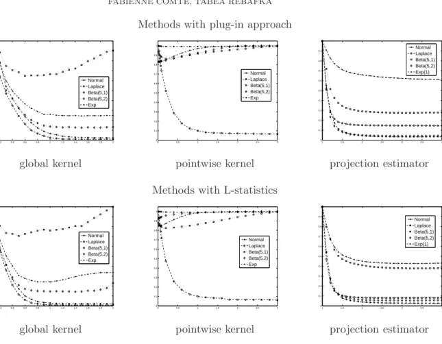
Figure 1. (rescaled) MISE for all estimators as a function ofκfor different
distributions off.
This problem arises with data in time-resolved fluorescence, where only the shortest arrival time of a group of photons can be observed (O’Connor and Phillips, 1984). Here it is assumed that the size N of a group of photons follows the Poisson distribution restricted to N∗ with known parameter µ. The renormalized probability masses are given by P(N =
k) = µk/k!/(eµ−1). As µ is known, the link function H is known as well with M(u) = (eµu−1)/(eµ−1). We see that the pile-up model is a special case of model (1) and model assumptions (5) and (6) are fulfilled witha=µ/(eµ−1),d=µeµ/(eµ−1) andb=µ2/(1−
e−µ). Furthermore, the weight function is given byw(u) = (1−e−µ)/[µ(u(e−µ−1) + 1)].
5.2. Computational issues and calibration. We implemented the adaptive pointwise kernel estimators ˆfˆ(i)
hi(x0)(x0), i= 1,2 defined by (16) with ˆhi(x0) given by (15), the adaptive
global kernel estimators ˆfˆ(i)
h(i), i= 1,2 given by (17)-(19) as well as the adaptive projection
estimators ˆf(i)
ˆ
m(i), i= 1,2 described in Section 3.3.
In the following simulations the bandwidth collection (C2) is used for the kernel estima-tors. Indeed, collections (C1) and (C3) are much larger, without leading to proportionally better results. For the kernel estimators we used the gaussian kernel, i.e. K(u) = e−u2
gl k L gl k P p k L p k P proj L proj P 0 0.005 0.01 0.015 0.02 0.025 0.03 0.035 0.04 Normal(10,1) distribution gl k L gl k P p k L p k P proj L proj P 0 0.05 0.1 0.15 0.2 0.25 Laplace(3,10) distribution gl k L gl k P p k L p k P proj L proj P 0 0.2 0.4 0.6 0.8 1 1.2 1.4 1.6 1.8 Beta(5,1) distribution gl k L gl k P p k L p k P proj L proj P 0 0.1 0.2 0.3 0.4 0.5 0.6 Beta(5,2) distribution gl k L gl k P p k L p k P proj L proj P 0 0.2 0.4 0.6 0.8 1 1.2 1.4 Exponential(1) distribution
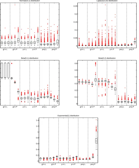
Figure 2. Each boxplot represents the values of MISE*1000 of the six
esti-mators computed on 1000 datasets for 5 different distributions withn= 500 and for µ= 0.1,0.8,2 (from left to right in the figure).
In the quantitiesV0(i)(h), i= 1,2 the value ofkfk∞resp. kgk∞is replaced by estimators. More precisely, kgk∞ is approximated by the 95th percentile of {maxx0gˆh(x0), h ∈ H}.
Likewise, kfk∞ is approximated by the 95th percentile of{maxx0fˆ (2)
h (x0), h∈ H}.
The terms kθˆ(h,hi)′ −θˆ
(i)
h′k2, i= 1,2 in (18) are approximated by Riemann-type
Normal N(10,1) distribution Laplace L(10,3) distribution µ 0.1 0.8 2 0.1 0.8 2 n 500 2000 500 2000 500 2000 500 2000 500 2000 500 2000 gl. ker L 3.08 2.76 3.09 2.59 3.23 2.67 1.76 0.940 1.14 0.579 1.22 0.416 gl. ker P 3.09 2.77 3.37 2.80 5.60 4.66 1.93 1.07 2.00 1.44 2.28 1.42 p. ker L 3.09 2.68 3.09 2.65 3.26 2.70 5.50 3.33 4.16 2.66 3.81 1.88 p. ker P 3.10 2.68 3.32 2.83 5.62 4.70 5.70 3.43 5.07 3.51 4.41 2.77 proj L 1.82 0.421 1.83 0.433 2.26 0.617 3.82 2.72 3.92 2.77 4.24 2.87 proj P 1.83 0.426 2.25 0.482 4.03 1.18 3.98 2.89 7.21 6.20 26.2 27.4
BetaB(5,1) distribution Beta B(5,2) distribution
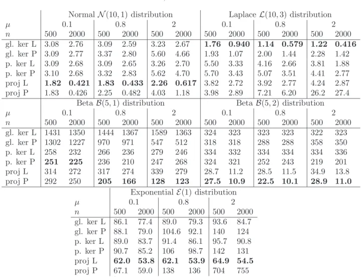
µ 0.1 0.8 2 0.1 0.8 2 n 500 2000 500 2000 500 2000 500 2000 500 2000 500 2000 gl. ker L 1431 1350 1444 1367 1589 1363 324 323 323 323 322 323 gl. ker P 1302 1227 970 971 547 512 318 318 288 288 358 350 p. ker L 258 232 266 236 279 246 334 332 334 334 334 336 p. ker P 251 225 236 210 247 268 324 321 252 243 219 201 proj L 314 272 317 274 339 279 28.7 11.2 28.5 11.5 34.9 13.8 proj P 292 250 205 166 128 123 27.5 10.9 22.5 10.1 28.9 11.0 Exponential E(1) distribution µ 0.1 0.8 2 n 500 2000 500 2000 500 2000 gl. ker L 86.1 77.4 89.0 79.3 93.6 84.7 gl. ker P 88.1 79.0 104.6 92.1 140 124 p. ker L 89.0 83.7 91.4 86.1 95.7 90.8 p. ker P 90.7 85.2 106 98.7 142 131 proj L 62.0 53.8 62.1 53.9 64.9 54.5 proj P 67.1 59.0 138 136 704 755
Table 1. Mean MISE*1000 values for the six different estimators in 30
different settings.
We noted that the projection estimators are much improved by normalizing ˆf(i)
ˆ
m(i), i= 1,2
such that its integral equals one. However, normalization is only appropriate when the interval where the density is estimated covers the main support of the density. For the kernel estimators normalization does not seem to be necessary. In fact, the property is almost automatic ifK is a density because thenR ˆ
fh(x)dx= (1/n)Pni=1w(i/n)≃
R1
0 w(u)du= 1.
The different penalty constantsκ(ji)are calibrated via simulation. For every estimator the mean integrated squared error kfˆ−fk2 is approximated on a grid ofκ-values for different
distributions. The aim is to choose κ such that the MISE is minimized simultaneously for all distributions.
Figure 1 represents the results for the following five distributions forf: normalN(10,1), LaplaceL(10,3), BetaB(5,1), BetaB(5,2) and exponentialE(1) distribution. The Poisson parameter is set toµ= 0.8. For every point of the grid of κ-values, 1000 datasets of sample size 500 are generated, and the 6 estimators and the associated MISE are evaluated. The mean values of the MISE are represented in Figure 1. For the sake of readability, the MISE curves are rescaled such that they are contained in the interval [0,1]. Recall that only the point matters where the MISE attains the minimum, and not the value of the minimum.
One observes that the MISE curves for the methods based on L-statistics (first row) and the plug-in method (second row) are always quite similar. Hence, the same κ may be used for both methods, i.e. κ(1)j = κ(2)j for j = 1,2,3. However, the MISE curves are quite different from one estimation strategy to another.
The global kernel estimators as well as the projection estimators are rather robust with regard to the choice of κ, as there exists an interval ofκ-values where all MISE curves are quite flat and achieve there minimum. In the following we set κ(1)1 = κ(2)1 = 1.1 for the global kernel estimators and κ(1)2 =κ(2)2 = 3 for the projection estimators.
Concerning the pointwise kernel estimators, the MISE is rather sensitive to the value of κ(0i). Slight changes may have a strong impact on the result. Furthermore, the estimators have quite the opposite behavior for the BetaB(5,1) and the Laplace distribution. For the former the minimum of the MISE is attained at κ(0i) = 0.09, for the latter at κ(0i) = 5 (the largest value of κ(0i) considered here). It is not clear which value of κ(0i) achieves the best compromise among all distributions. In the following we setκ(1)0 =κ(2)0 = 0.4.
5.3. Comparison of all six estimators. There are several factors potentially influencing the performance of the different estimators. In our simulation study we consider
• two different sample sizes (n= 500 andn= 2000),
• three levels of the Poisson parameter (µ= 0.1, µ= 0.8 and µ= 2),
• five different distributions: normal N(10,1), Laplace L(10,3), Beta B(5,1), Beta B(5,2), exponentialE(1),
giving a total of 30 settings.
To evaluate the performance of the estimators we proceed exactly as in the calibration study. For each setting the estimators and their MISE are evaluated on 1000 datasets. The boxplots in Figure 2 represent the corresponding results when the sample size is 500. Table 1 shows all means of the MISE in the different settings.
We now analyze the impact of the different factors on the performance of the estimators. Therefore, we study how the mean MISE evolves when one of the factors changes.
Impact of the sample size. As usual, increasing the sample size results in a decrease of the MISE. Interestingly, depending on the estimation strategy and on the type of distribution, this decrease can be more or less pronounced. The increase of the sample size is more ben-eficial for the projection estimators than for the kernel estimators. The improvement is by far more important for the normal distribution than for the BetaB(5,1) or the exponential distribution.
Impact of the Poisson parameter. In the pile-up model the Poisson parameter µis related to the degree of distortion. In other words, it represents the amount of bias in the model. The three levels ofµconsidered here correspond to a very low (µ= 0.1), medium (µ= 0.8) and high (µ= 2) degree of distortion. As increasing µresults in a more difficult estimation problem, we observe increasing MISE values in almost all settings, see Figure 2. However, there are some exceptions where the MISE decreases whenµincreases. We do not have any explanation for this phenomenon.
Comparison of estimation strategies: Global kernel, pointwise kernel or projection strategy?
Depending on the underlying target distribution there are significant differences in the performance of the different estimation strategies.
0 1 2 3 4 5 0 0.5 1 1.5 2 2.5 noise sample 0 1 2 3 4 5 6 7 8 0 0.05 0.1 0.15 0.2 0.25 0.3 0.35 data true density (a) (b) 0 0.5 1 1.5 2 2.5 3 3.5 4 0 0.05 0.1 0.15 0.2 0.25 0.3 0.35 kernel estim. projection estim. true density (c)
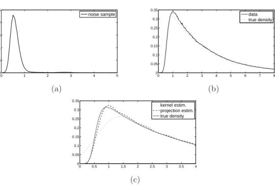
Figure 3. (a) Noise sample. (b) Fluorescence data and target density f.
(c) Estimators for fluorescence data and target density f.
Both projection methods are best for the normal distribution and the Beta B(5, 2)-distribution. For the BetaB(5,1)-distribution they perform similarly good as the pointwise kernel methods. However, in the exponential case there is a stark difference between the projection estimator based on L-statistics, which is best in all settings, and the projection plug-in estimator being by far the worst method for largeµ.
The global kernel estimators are best in the Laplace case, and do generally well, except for the Beta distributions.
Pointwise kernel estimators are traditionally known to be well adapted to capture peaks like in the exponential or Laplace distribution. Here, we cannot observe this property, since in almost all settings global strategies (kernel and projection) are doing better.
Consequently, there is no estimation strategy that outperforms the others in all set-ups, but a preference should be given to projection strategies and global kernel estimators.
Comparison of bias correction approaches: L-statistics or plug-in strategy? When µ= 0.1 there is almost no bias in the model. Consequently, no significant difference between the methods is observed. However, for largerµ, differences in the MISE appear for the different bias correction methods. Increasing namplifies the difference between the methods.
Depending on the type of distribution, one or the other correction approach is preferable. In the case of the normal, Laplace and the exponential distribution, all estimators using L-statistics always lead to better results than the corresponding plug-in estimators. However, in the case of the Beta distributions, the plug-in versions mostly give better results. 5.4. Application to real data. We now apply our statistical methods to real fluorescence lifetime measurements. The data are supposed to be generated by the pile-up model with Poisson parameter µ = 0.166. The target density f is known to be the convolution of an exponential density fE with mean 2.54 ns and some positive noise fη coming from the measuring instrument, i.e. f =fη⊗fE. The noise densityfη can be observed separately, so
that we assume thatfη is a known function. Figure 3(a) gives a histogram of an independent noise sample of size 259,386. Note that the same dataset has already been analyzed in ?, but from a deconvolution point of view, that is the aim was the recovery of the exponential density fE. Here we are interested in the estimation of f =fη⊗fE.
Figure 3(b) shows the data in form of a histogram with very fine bins and target densityf. The sample size is 17,402. Here we clearly observe the pile-up effect, that is the histogram is biased in the sense that mass is shifted to the origin compared to the original density f. On this dataset the pointwise and global kernel estimators coincide for both strategies (L-statistics and plug-in). The two projection estimators differ only slightly. For illustration, Figure 3(c) displays the plug-in projection estimator and the global kernel estimator based on L-statistics compared to density f. We can see that the projection estimator gives a very good recovery of the target density f, whereas the kernel estimator seems to do too much bias correction. Indeed, the corresponding squared errors kf−fˆk2 are given by
kernel estimator using L-statistics (pointwise and global) 6.056 10−3 kernel estimator by plug-in (pointwise and global) 6.214 10−3
projection estimator using L-statistics 0.433 10−3 projection estimator by plug-in 0.431 10−3 .
Consequently the plug-in projection estimator gives the best approximation.
6. Appendix
6.1. Proof of Proposition 4.1. Let x0 be a fixed point. Denote by ˇfh the pseudo-estimator of f given by ˇfh(x) = n1Pni=1w◦G(Zi)Kh(x−Zi). We write
(30) fˆh(2)(x0)−f(x0) = ˆ fh(2)−fˇh (x0) + ˇfh−E[ ˇfh] (x0) + E[ ˇfh]−f (x0).
First, we state that by property (7) we have
(31) E[ ˇfh(x0)] =E[Kh(x0−Yi)] =Kh∗f(x0) =:fh .
The last term in (30) is a standard bias term in kernel density estimation (Tsybakov, 2004)). Denote b(x) = E[ ˇfh]−f(x). As R K(u)du= 1, b(x0) = Z Kh(x0−y)f(y)dy−f(x0) = Z K(u) [f(x0−uh)−f(x0)] du .
By a standard Taylor expansion of f, we get (see e.g. Tsybakov (2004))
(32) |b(x0)| ≤ CR |x|β|K(x)|dx ℓ! h β =C 1hβ .
To study the second term of (30), we successively apply property (7), 0≤w≤1/aand the fact that K is square-integrable to obtain
Eh fˇh−E( ˇfh)2(x0)i = 1 nVar (w◦G(Z1)Kh(x0−Z1))≤ 1 nE h {w◦G(Z1)Kh(x0−Z1)}2 i ≤ 1 anE h Kh(x0−Y1)2 i = 1 anh2 Z K2 x0−y h f(y)dy ≤ anh1 kfk∞kKk22 . (33)
For the first term in decomposition (30), the Lipschitz property ofw implies that E ˆ fh(2)−fˇh 2 (x0) ≤ c 2 w n n X i=1 E h ( ˆGn−G)2(Zi)Kh2(x0−Zi) i = c 2 w n n X i=1 E " ˆ Gn,i− n−1 n G 2 (Zi)Kh2(x0−Zi) # +E " 1 n(1−G(Zi)) 2 Kh2(x0−Zi) #! , since the cross product term is centered, where ˆGn,i(x) =n−1Pnj=1,j6=i1Zj≤x. Then
E " ˆ Gn,i− n−1 n G 2 (Zi)Kh2(x0−Zi) # =E " E " ˆ Gn,i− n−1 n G 2 (Zi)Kh2(x0−Zi) Zi ## =E n−1 n2 G(Zi)(1−G(Zi))K 2 h(x0−Zi) ≤ 1 4nE Kh2(x0−Zi)≤ k gk∞kKk2 2 4nh . Therefore, as kgk∞ ≤dkfk∞ andcw ≤b/a3, we obtain that
E ˆ fh(2)−fˇh 2 (x0) ≤ 5db 2 4nha6kfk∞kKk 2 2 . (34)
Gathering (32), (33) and (34) yields the result. 6.2. Proof of Proposition 4.2. By (30) it follows that
E h kfˆh(2)−fk22 i ≤3E h kfˆh(2)−fˇhk22 i +Ekfˇh−E[ ˇfh]k22+kE[ ˇfh]−fk22 . (35)
Concerning the last term of (35), proceeding as in Tsybakov (2004), we get
(36) kE[ ˇfh]−fk2 2 ≤ Lhβ (ℓ−1)! Z |K(u)||u|βdu 2 . For the first right-hand-side term of (35) we obtain
Ehkfˆ(2) h −fˇhk22 i = Z E 1 n n X i=1 w◦Gˆn(Zi)−w◦G(Zi) Kh(x−Zi) !2 dx ≤ Z E w◦Gˆn(Z1)−w◦G(Z1) 2 Kh2(x−Z1) dx ≤ c 2 w h kKk 2 2 E ˆ Gn(Z1)−G(Z1) 2 ≤ b 2 nha6kKk 2 2, (37)
where we used thatE[( ˆGn(Z1)−G(Z1))2]≤1/n. This property can be shown by proceeding
as in the pointwise case and using that G(Z1) has uniform distribution.
For the second term of (35) we obtain
E kfˇh−E[ ˇfh]k22 = 1 n Z Ehw◦G(Y1) (Kh(x−Y1))2idx ≤ 1 an Z Z (Kh(x−y))2dxf(y)dy = 1 anhkKk 2 2 . (38)
Combining (36), (37) and (38) completes the proof.
6.3. Proof of Theorem 4.1. For the sake of readability, super-indices (2) are omitted in
the whole proof. For anyh∈ H,
ˆ fˆh(x0)−f 2 (x0)≤3 ˆ fhˆ(x0)−fˆh,ˆh(x0) 2 (x0) + ˆ fh,ˆh(x0)−fˆh 2 (x0) + ˆ fh−f 2 (x0) ≤3 A0(h, x0) +V0(ˆh(x0)) +A0(ˆh(x0), x0) +V0(h) +fˆh−f 2 (x0) ≤6A0(h, x0) + 6V0(h) + 3 ˆ fh(x0)−f(x0) 2 , (39)
where the second inequality holds by the definition of A0, i.e. for all h, h′ ∈ H we have
A0(h, x0) +V0(h′) ≥
ˆ
fh,h′(x0)−fˆh′(x0)
2
. The last inequality holds by the definition of ˆh(x0), that is A0(ˆh(x0), x0) +V0(ˆh(x0)) ≤ A0(h, x0) +V0(h) for all h ∈ H. The term E[( ˆfh(x0)−f(x0))2] is controlled by Proposition 4.1. Hence, it is sufficient to study the
termE[A0(h, x0)]. We state that
(40) A0(h, x0) = sup h′∈H ˆ fh,h′(x0)−fˆh′(x0) 2 −V0(h′) + ≤5 (D1+D2+D3+D4+D5) , where D1= sup h′∈H ˆ fh,h′(x0)−fˇh,h′(x0) 2 , D2 = sup h′∈H ˇ fh,h′(x0)−E ˇ fh,h′(x0) 2 −V010(h′) + , D3= sup h′∈H Efˇh,h′(x0)−Efˇh′(x0)2 , D4 = sup h′∈H Efˇh′(x0)−fˇh′(x0)2−V0(h ′) 10 + , and D5= sup h′∈H ˇ fh′(x0)−fˆh′(x0) 2 , with ˇfh,h′ =Kh′ ∗fˇh.
We start with term D3. Recall that E[ ˇfh(x0)] = Kh ∗f(x0) by (31). Likewise, by
property (7),Efˇh,h′(x0)=Kh′∗Kh∗f(x0).In general we haveks∗rk∞≤ ksk∞krk1 and
kKhk1=kKk1, yielding
E
ˇ
fh,h′(x0)−Efˇh′(x0)=|Kh′ ∗(Kh∗f−f)(x0)| ≤ kKh∗f−fk∞kKk1 .
Now remark that (Kh∗f −f) (x) =b(x) is the pointwise bias term considered in the proof of Proposition 4.1 Hence, (32) yields
(41) D3≤C12kKk21h2β .
Concerning term D4 we note that
E[D4]≤X h∈H E ˇ fh(x0)−E ˇ fh(x0) 2 −V0(h) 10 + =X h∈H Z ∞ 0 P ˇ fh(x0)−Efˇh(x0) 2− V0(h) 10 + > x dx =X h∈H Z ∞ 0 P fˇh(x0)−E ˇ fh(x0) > r V0(h) 10 +x ! dx .
The probability in the last term can be bounded by the Bernstein inequality. To this end we introduce the random variablesSi=w◦G(Zi)Kh(x0−Zi). Obviously,|Si| ≤ kKk∞/(ah) =:
M almost surely and by property (7)
Var (Si)≤Ew2◦G(Z1)Kh2(x0−Z1)=Ew◦G(Y1)Kh2(x0−Y1)≤ k
Kk2 2kfk∞
ah =:v . Hence, the Bernstein inequality implies for any x >0
P fˇh(x0)−E ˇ fh(x0) ≥ r V0(h) 10 +x ! =P 1 n n X i=1 (Si−E[Si]) ≥ r V0(h) 10 +x ! ≤2 max ( exp −n 4v V0(h) 10 +x ,exp −nα 4M r V0(h) 10 ! exp −n(1−α) 4M √ x ) , for any α∈[0,1] as√·is a concave function. By the definition ofV0(h)
n 4v V0(h) 10 = κ0kKk21logn 40 ≥plogn , forκ0≥40p, sincekKk21≥1. Furthermore,
nα 4M r V0(h) 10 = αkKk2kKk1 4kKk∞ r κ0akfk∞hnlogn 10 =ρα p hnlogn≥plogn , for nh≥(p2/ρ2
α) logn. We can choose α∈[0,1] sufficiently close to 0 such that p/ρα >1. Then the inequality in the last display holds under (H3), yielding
E[D4]≤ X h∈H Z ∞ 0 2n−pmax exp − nhax 4kKk2 2kfk∞ ,exp −(1−α)nha √ x 4kKk∞ dx ≤2n−p X h∈H Z ∞ 0 maxne−τ1nhx,e−τ2nh√xodx≤2n−pX h∈H max 1 τ1 , 2 τ2 2 ≤C′n−p+1,
ash≥1/nand the cardinality of Hverifies #H ≤n. Finally, we choose p= 2 to get (42) E[D4]≤ C
′
n .
TermD2 can be treated in exactly the same way as D4. More precisely, instead ofSi use Ti=w◦G(Zi)Kh∗Kh′(Zi−x0) verifying ˇ fh,h′(x0)−E ˇ fh,h′(x0) = 1 n n X i=1 Ti−E[Ti],
and |Ti| ≤ kKk∞kKk1/(ah′) =: ¯M and Var(T1)≤ kfk∞kKk21kKk22/(ah′) =: ¯v. Hence, the
Bernstein inequality yields
(43) E[D2]≤ C
′′
n .
Lemma 6.1. Under the assumptions (H2) and (5), for any set Ω and for all t∈R, E ˆ fh(t)−fˇh(t) 2 1Ωc ≤c2wkKk2∞n2P(Ωc) and E ˆ fh′,h(t)−fˇh′,h(t) 2 1Ωc ≤c2wkKk2∞kKk21n2P(Ωc) .
Proof. By usingkGˆn−Gk∞≤1, we have
E ˆ fh(t)−fˇh(t) 2 1Ωc =E 1 n n X i=1 (w◦Gˆn(Zi)−w◦G(Zi))Kh(t−Zi) !2 1Ωc ≤ c 2 w n2E n X i=1 |Kh(t−Zi)| !2 1Ωc ≤c2wE Kh2(t−Z1)1Ωc ≤c2wkKhk2∞E[1Ωc] = c 2 w h2kKk 2 ∞P(Ωc)≤c2wkKk2∞n2P(Ωc) ,
as 1/h ≤ n. In the same way, we show the second statement of the Lemma, by using kKh′∗Khk∞≤ kKh′k∞kKhk1 ≤nkKk∞kKk1.
Now let Ω ={ω:kGˆn−Gk∞≤s}for some constant s >0. Then (see Massart (1990)),
(44) P(Ωc) =P(kGˆn−Gk∞> s)≤e−2ns2 ,
by the Dvoretzky-Kiefer-Wolfowitz inequality. This implies that
E sup h∈H ˆ fh(x0)−fˇh(x0) 2 1Ωc ≤X h∈H E ˆ fh(x0)−fˇh(x0) 2 1Ωc ≤ X h∈H c2wkKk2∞n2e−2ns2 =c2wkKk2∞n3e−2ns2 <∞, as #H ≤n. Furthermore, E sup h∈H ˆ fh(x0)−fˇh(x0) 2 1Ω ≤c2wE sup h∈H 1 n n X i=1 |Gˆn(Zi)−G(Zi)||Kh(x0−Zi)| !2 1Ω ≤s2c2wE sup h∈H 1 n n X i=1 |Kh(x0−Zi)| !2 ≤2s2c2w E sup h∈H 1 n n X i=1 (|Kh(x0−Zi)| −E[|Kh(x0−Zi)|]) !2 + sup h∈H E " 1 n n X i=1 |Kh(x0−Zi)| #!2 ≤2s2c2w ( 1 n X h∈H Var (|Kh(x0−Z1)|) + sup h∈H [E(|Kh(x0−Z1)|)]2 ) . On the one hand,
1 n X h∈H Var (|Kh(x0−Z1)|)≤ 1 n X h∈H EKh2(x0−Z1)= 1 n X h∈H 1 hkKk 2 2kgk∞≤SkKk22dkfk∞,
where S is defined in (H3) anddin (6). On the other hand, sup h∈H [E(|Kh(x0−Z1)|)]2 = sup h∈H Z |K(z)|g(x0−zh)dz 2 ≤d2kfk2∞kKk21 .
It follows that E[D5] ≤ µ1n3e−2ns2 + µ2s2, with constants µ1 = c2wkKk2
∞ and µ2 =
2c2
wdkfk∞(SkKk22+dkfk∞kKk21). Choosing s2= 2 logn/n gives
(45) E[D5]≤ µ1
n + 2µ2 logn
n .
Finally, the study of D1 follows the same line as the study of D5. That is, on the one
hand, we have for the same set Ω
E[D11Ωc]≤c2wkKk2
∞kKk21n3e−2ns 2
. On the other hand,
E[D11Ω]≤2s2c2 w ( 1 n X h∈H E (Kh′ ∗Kh(x0−Z1))2+ sup h∈H (E[|Kh′∗Kh(x0−Z1)|])2 ) . By the generalized Minkowski inequality, we obtain
E(Kh′∗Kh(x0−Z1))2≤ " Z |Kh′(u)| Z Kh2(x0−z−u)g(z)dz 1/2 du #2 ≤ kgk∞kKhk22kKh′k21 ≤dkfk∞kKk22kKk21/h . Furthermore, sup h∈H (E[|Kh′∗Kh(x0−Z1)|])2≤ sup h∈H Z Z Kh′(u) Z |K(v)|g(x0−vh−u)dvdu 2 ≤(dkfk∞kKk21)2 .
It follows with ˜µ1=µ1kKk21 and ˜µ2 =µ2kKk12 that E[D1]≤µ˜1n3e−2ns 2 + ˜µ2s2. Hence, (46) E[D1]≤ µ˜1 n + 2˜µ2 logn n ,
withs2 = 2 logn/n. Now, if we plug (41), (42), (43), (45) and (46) into (40), we get
E[A0(h, x0)]≤C˜1h2β + ˜C2logn
n ,
which, associated with Proposition 4.1, can be inserted in (39) to end the proof of Theorem 4.1.
6.4. Proof of Theorem 4.2. In all the proof below, super-indices(2)are omitted. Similar to the pointwise case, we have for any h∈ H
kfˆhˆ−fk22≤6A(h) + 6V(h) + 3kfˆh−fk22 .
(47)
By the proof of Proposition 4.2,
Ehkfˆh−fk22i≤3kfh−fk22+C4
nh . (48)
Hence, only term E[A(h)] needs to be studied. By analogy to the proof of Theorem 4.1,
A(h)≤5(F1+F2+F3+F4+F5),
where F1= sup h′∈Hk ˆ fh,h′−fˇh,h′k22 , F2 = sup h′∈H kfˇh,h′−E[ ˇfh,h′]k22− V(h′) 10 + , F3= sup h′∈Hk E[ ˇfh,h′]−E[ ˇfh′]k22, F4 = sup h′∈H kE[ ˇfh′]−fˇh′k22−V(h ′) 10 + , F5= sup h′∈Hk ˇ fh′−fˆh′k22.
First, we study term F3. The inequalityku∗vk2≤ kuk1kvk2 yields
(50) F3 = sup
h′∈Hk
Kh′∗Kh∗f−Kh′∗fk22 ≤ sup
h′∈Hk
Kh′k21kKh∗f −fk22 =kKk21kf −fhk22 .
To study term F4 we introduce the centered empirical processνn,h defined by νn,h(ψ) =hfˇh−E[ ˇfh], ψi = 1 n n X i=1 Z (w◦G(Zi)Kh(u−Zi)−E[w◦G(Zi)Kh(u−Zi)])ψ(u)du . As ψ 7→ νn,h(ψ) is continuous, the supremum can be taken over a countable dense subset of {ψ ∈ L2,kψk = 1}, which we denote by B(1). Then, kfˇh −E[ ˇfh]k2
2 = supψ∈B(1)hfˇh − E[ ˇfh], ψi2 = sup ψ∈B(1)νn,h(ψ). Therefore we obtain E[F4]≤ X h∈H E kfˇh−E[ ˇfh]k22− V(h) 10 + =X h∈H E " sup ψ∈B(1) νn,h2 (ψ)−V(h) 10 ! + # . The expectation in the last term can be bounded by Talagrand’s inequality (see Sub-section 6.7). More precisely, to apply this result, we have to determine the values of the constants H, M and v. Denote fψ(z) = w ◦ G(z)Kh ∗ ψ(z), so that νn,h(ψ) =
1
n
Pn
i=1(fψ(Zi)−E[fψ(Zi)]). First, for any ψ∈ B(1) the Cauchy-Schwarz inequality gives kfψk∞≤ 1akKh∗ψk∞= a1sup z |h|Kh(· −z)|,|ψ|i| ≤ kKhk2kψk2 a ≤ kKk2 a√h =:M . Next, we see that
E " sup ψ∈B(1)| νn,h(ψ)| #!2 ≤E " sup ψ∈B(1) νn,h2 (ψ) # ≤Ekfˇh−E[ ˇfh]k22≤ V(h) κ1 =:H2 ,
by (38). Furthermore, let ε2= 1/2. To obtain 4H2 =V(h)/10, we setH =p
V(h)/40. Lastly, for any ψ∈ B(1) we show that by (7)
Var (fψ(Z))≤E (w◦G(Z)Kh∗ψ(Z))2 ≤ 1a Z (Kh∗ψ(y))2f(y)dy ≤ 1akfk∞kKh∗ψk22 ≤ 1 akfk∞kKhk 2 1kψk22 ≤ 1 akfk∞kKk 2 1=:v .
Finally, Talagrand’s inequality yields
E " sup ψ∈B(1) νn,h2 (ψ)−V(h) 10 ! + # ≤ C˜1 n e−C˜2/h+ 1 nhe −C˜3√n ≤ C˜1 n e −C˜2/h+C˜4 n ! ,
where ˜Ck>0, k= 1, . . . ,4 are constants depending on K,kfk∞ and a. Consequently, (51) E[F4]≤ C˜1 n X h∈H e−C˜2/h+ C˜4 n ! ≤ C˜n5 , as #H ≤nand P h∈He− ˜ C2/h≤Σ(C′ 2) under condition (26).
In the same way we obtain for F2
(52) E[F2]≤ C¯
n . Now let us turn toF5. We note that
kfˆh−fˇhk22≤ 4 a2n2 Z n X i=1 |Kh(u−Zi)| !2 du≤ 4 a2n n X i=1 kKh(· −Zi)k22= 4 a2hkKk 2 2≤ 4n a2kKk 2 2. Therefore, E sup h∈Hk ˆ fh−fˇhk221Ωc ≤ 4na2kKk22P(Ωc),
where Ω ={ω :kG−Gˆnk∞≤s} as previously, and we recall that P(Ωc)≤e−2ns
2
. Following the same line as for D5 in the pointwise case and by choosing s=
p logn/n, we conclude that (53) E[F5]≤ C ′ 1 n +C2′ logn n . For F1, we follow the same line as for F5 to obtain
(54) E[F1]≤ kKk21 C1′ n +C ′ 2 logn n .
Consequently, plugging (50), (51), (52), (53) and (54) into (49) gives a bound of E[A(h)].
Combining this with (48), (47) and the definition of V(h) yields Theorem 4.2.
6.5. Proof of Proposition 4.3. Pythagoras formula yieldskf−fˆmk22 =kf−fmk22+kfm− ˆ
fmk22.By definition of the orthogonal projectionfm=P2jm=0ajϕj and by using equality (7), we have aj =hϕj, fi =E(ϕj(Y)) =E(ϕj(Z1)w◦G(Z1)).This, together with formula (13)
implies thatkfm−fˆmk22= P2m j=0(aj −ˆaj)2.If we define (55) νn(h) = 1 n n X i=1 [h(Zi)w◦G(Zi)−E(h(Zi) w◦G(Zi))], (56) Rn(h) = 1 n n X i=1 h(Zi)[w◦Gˆn(Zi)−w◦G(Zi)], then we get kfm−fˆmk22 ≤2 P2m
j=0(νn(ϕj)2+Rn(ϕj)2).We have, on the one hand,
2m X j=0 E(ν2 n(ϕj)) = 2m X j=0 1 nVar(ϕj(Zi)w◦G(Zi))≤ 2m X j=0 1 nE ϕ2j(Z1)(w◦G(Z1))2 ≤ 1 nE k 2m X j=0 ϕ2jk∞(w◦G(Z1))2 ≤ Dm n E[(w◦G(Z1)) 2]≤ 1 a2 Dm n , (57)
because the basis satisfiesP2m
j=0ϕ2j = 2m+ 1 =Dm. On the other hand, we have
2m X j=0 E(R2 n(ϕj))≤ 2m X j=0 E 1 n n X i=1 ϕj(Zi)[w◦Gˆn(Zi)−w◦G(Zi)] !2 ≤ 1 n n X i=1 2m X j=0 E ϕ2j(Zi)[w◦Gˆn(Zi)−w◦G(Zi)]2 ≤c2w 2m X j=0 E kG−Gˆnk2∞ϕ2j(Zi) ≤c2wDmE kG−Gˆnk2∞ ≤c2wDm n , (58)
with (5) and because ofEkG−Gˆnk2
∞
≤1/n (see e.g. Brunel and Comte, 2005, p. 462). By gathering all terms, we obtain the risk bound stated in Proposition 4.3.
6.6. Sketch of proof of Theorem 4.3. In the following, we omit the super index(2).
It is easy to see that ˆfm = arg mint∈Smγn(t) forγn(t) =ktk
2−2n−1Pn
i=1w◦Gˆn(Zi)t(Zi). Thus, we can write γn(t)−γn(s) =kt−fk22− ks−fk22−2νn(t−s)−2Rn(t−s),where νn and Rn are defined by (55) and (56). By definition of ˆfmˆ we have for all m ∈ Mn, γn( ˆfmˆ) + pen( ˆm)≤γn(fm) + pen(m). This can be rewritten askfˆmˆ −fk22 ≤ kfm−fk22+
pen(m) + 2νn( ˆfmˆ−fm)−pen( ˆm) + 2Rn( ˆfmˆ−fm).Using this and and that 2xy≤x2/θ+θy2 for all nonnegative x, y, θ, we obtain
kf−fˆmˆk22≤ kf−fmk22+ pen(m) + 2νn( ˆfmˆ −fm)−pen( ˆm) + 2Rn( ˆfmˆ −fm) kf −fˆmˆk22 ≤ kf −fmk22+ pen(m) + 2kfˆmˆ −fmk2 sup t∈Smˆ+Sm,ktk2=1 |νn(t)| −pen( ˆm) + 2kfˆmˆ −fmk2 sup t∈Smˆ+Sm,ktk2=1 |Rn(t)| ≤ kf −fmk22+ pen(m) + 1 4kfˆmˆ −fmk 2 2+ 2 sup t∈Smˆ+Sm,ktk2=1 [νn(t)]2 −pen( ˆm) +1 8kfˆmˆ −fmk 2 2+ 8 sup t∈Smˆ+Sm,ktk2=1 [Rn(t)]2. Askfˆmˆ −fmk22≤2(kfˆmˆ −fk22+kfm−fk22), this yields 1 4E[kf−fˆmˆk 2 2] ≤ 7 4kf−fmk 2 2+ 2pen(m) + 8E sup t∈Smn,ktk2=1 [Rn(t)]2 ! +4E sup t∈Smˆ+Sm,ktk2=1 [νn(t)]2−(pen(m) + pen( ˆm))/4 ! + .
Then the term Esupt
∈Smˆ+Sm,ktk2=1[νn(t)]
2−(pen(m) + pen( ˆm))/4
+ is bounded by
C/n by using Talagrand Inequality in a standard way (see e.g. Brunel et al., 2005). For the last termE supt∈Smn,ktk2=1[Rn(t)]2 , we define ΩG by (59) ΩG={√nkGˆn−Gk∞≤ p log(n)}.
As in (44), we use Massart (1990) and get
(60) P(√nkGˆn−Gk∞ ≥λ)≤2e−2λ2.
This implies that P(Ωc
G) ≤ 2/n2. Then we write that E
supt∈S mn,ktk2=1[Rn(t)] 2 is less than E sup t∈Smn,ktk2=1 [Rn(t)1ΩG] 2 ! +E sup t∈Smn,ktk2=1 [Rn(t)1Ωc G] 2 ! :=R1+R2.
For the first term, we have
R1 ≤ c2wE " kGˆn−Gk2∞1ΩGE sup t∈Smn,ktk2=1 (1 n n X i=1 |t(Zi)|)2 !# ≤ c2wlog(n) n E t∈Smnsup,ktk2=1( 1 n n X i=1 t2(Zi)) ! ≤ 2c2wlog(n) n " E sup t∈Smn,ktk2=1 |νn′(t2)| ! + sup t∈Smn,ktk2=1 E(t2(Z1)) # where νn′(t) = n1Pn
i=1(t(Zi)−E(t(Z1)). It is proved in Brunel and Comte (2005) that E
supt∈S
mn,ktk2=1|νn′(t
2)|≤Clog(n) if the density ofZ
1 is bounded andNn≤O(√n) for the trigonometric basis. MoreoverE(t2(Z1))≤ ktk2
2kfk∞/w0. We obtainR1 ≤Clog2(n)/n.
On the other hand, we have R2 ≤ X j E(R2 n(ϕj)1Ωc)≤c2 wnE1/2(kGˆn−Gk4∞)P1/2(ΩcG)≤ C n. This yields Esupt
∈Smn,ktk2=1[Rn(t)]
2 ≤ Clog2(n)/n. Finally we obtain that, for all
m ∈ Mn, E[kf −fˆmˆk22] ≤ 7kf −fmk22 + 8pen(m) +Klog2(n)/n, which ends the proof.
6.7. The Talagrand inequality. The following result follows from the Talagrand concen-tration inequality given in (Klein and Rio, 2005) and arguments in (Birg´e and Massart, 1998) (see the proof of their Corollary 2 page 354).
Lemma 6.2. (Talagrand’s inequality) Let Y1, . . . , Yn be independent random variables, let νn,Y(f) = (1/n)Pni=1[f(Yi)−E(f(Yi))]and let F be a countable class of uniformly bounded
measurable functions. Then for ǫ2 >0
E h sup f∈F| νn,Y(f)|2−2(1 + 2ǫ2)H2 i + ≤ 4 K1 v ne −K1ǫ2nH 2 v + 98M 2 K1n2C2(ǫ2) e− 2K1C(ǫ2)ǫ 7√2 nH M , with C(ǫ2) =√1 +ǫ2−1, K 1 = 1/6, and sup f∈Fk fk∞≤M, E h sup f∈F| νn,Y(f)| i ≤H, sup f∈F 1 n n X k=1 Var(f(Yk))≤v.
By standard denseness arguments, this result can be extended to the case where F is a unit ball of a linear normed space, after checking that f 7→ νn(f) is continuous and F contains a countable dense family.
References
Asgharian, M., M’Lan, C. E., and Wolfson, D. B. (2002). Length-biased sampling with right censoring: an unconditional approach. J. Amer. Statist. Assoc., 97(457):201–209. Barron, A., Birg´e, L., and Massart, P. (1999). Risk bounds for model selection via
penal-ization. Probability Theory and Related Fields, 113:301–413.
Birg´e, L. and Massart, P. (1998). Minimum contrast estimators on sieves: exponential bounds and rates of convergence. Bernoulli, 4(3):329–375.
Brunel, E. and Comte, F. (2005). Penalized contrast estimation of density and hazard rate with censored data. Sankhya, 67:441–475.
Brunel, E., Comte, F., and Guilloux, A. (2005). Nonparametric density estimation in presence of bias and censoring. Test, 18:166–194.
Butucea, C. (2000). Two adaptive rates of convergence in pointwise density estimation.
Math. Methods Statist., 9(1):39–64.
Chesneau, C. (2010). Wavelet block thresholding for density estimation in the presence of bias. J. Korean Statist. Soc., 39(1):43–53.
Cutillo, L., De Feis, I., Nikolaidou, C., and Sapatinas, T. (2014). Wavelet density estimation for weighted data. J. Statist. Plann. Inference, 146:1–19.
de U˜na- ´Alvarez, J. (2004). Nonparametric estimation under length-biased sampling and type I censoring: a moment based approach. Ann. Inst. Statist. Math., 56(4):667–681. de U˜na- ´Alvarez, J. and Rodr´ıguez-Casal, A. (2006). Comparing nonparametric estimators
for length-biased data. Comm. Statist. Theory Methods, 35(4-6):905–919.
Donoho, D. L., Johnstone, I. M., Kerkyacharian, G., and Picard, D. (1996). Density esti-mation by wavelet thresholding. Annals of Statistics, 24:508–539.
Efromovich, S. (2004a). Density estimation for biased data. Ann. Statist., 32(3):1137–1161. Efromovich, S. (2004b). Distribution estimation for biased data.J. Statist. Plann. Inference,
124(1):1–43.
El Barmi, H. and Simonoff, J. S. (2000). Transformation-based density estimation for weighted distributions. J. Nonparametr. Statist., 12(6):861–878.
Gill, R. D., Vardi, Y., and Wellner, J. A. (1988). Large sample theory of empirical distri-butions in biased sampling models. Ann. Statist., 16(3):1069–1112.
Goldenshluger, A. and Lepski, O. (2011). Bandwidth selection in kernel density estimation: oracle inequalities and adaptive minimax optimality. Ann. Statist., 39(3):1608–1632. Jones, M. C. (1991). Kernel density estimation for length biased data. Biometrika,
78(3):511–519.
Klein, T. and Rio, E. (2005). Concentration around the mean for maxima of empirical processes. Annals of Probability, 33:1060–1077.
Li, X. and Zuo, M. J. (2004). Preservation of stochastic orders for random minima and maxima, with applications. Naval Research Logistics, 51(3):332–344.
Massart, P. (1990). The tight constant in the dvoretzky-kiefer-wolfowitz inequality. Annals of Probability, 18:1269–1283.
O’Connor, D. V. and Phillips, D. (1984). Time-correlated single photon counting. Academic Press, London.
Rebafka, T., Roueff, F., and Souloumiac, A. (2010). A corrected likelihood approach for the pile-up model with application to fluorescence lifetime measurements using exponential mixtures. The International Journal of Biostatistics, 6(1).
Shaked, M. and Wong, T. (1997). Stochastic comparisons of random minima and maxima.
Tsodikov, A. (2001). Estimation of survival based on proportional hazards when cure is a possibility. Mathematical and Computer Modelling, 33(12–13):1227–1236.
Tsybakov, A. B. (2004). Introduction `a l’estimation non-param´etrique, volume 41 of
Math´ematiques & Applications (Berlin) [Mathematics & Applications]. Springer-Verlag, Berlin.
Vardi, Y. (1982). Nonparametric estimation in the presence of length bias. Ann. Statist., 10(2):616–620.
Wu, C. O. (1997). A cross-validation bandwidth choice for kernel density estimates with selection biased data. J. Multivariate Anal., 61(1):38–60.
Wu, C. O. and Mao, A. Q. (1996). Minimax kernels for density estimation with biased data.