A Fuzzy Programming approach for
formation of Virtual Cells under dynamic
and uncertain conditions
R.Jayachitra
Lecturer, Department of Mechanical Engineering PSG College of Technology, Coimbatore
A.Revathy
PG Scholar, Department of Mechanical Engineering PSG College of Technology, Coimbatore
P.S.S.Prasad
Asst. Professor, Department of Mechanical Engineering PSG College of Technology, Coimbatore Abstract:
Inspired by principles and advantages of the group technology (GT) philosophy, part family formation for a virtual Cellular Manufacturing System (VCMS) using Fuzzy logic is designed for dynamic and uncertain conditions. In real manufacturing systems, the input parameters such as part demand and the capacity are fuzzy in nature. In such cases, the fluctuations in part demand and the availability of manufacturing facilities in each period can be regarded as fuzzy. In a dynamic environment, the planning horizon can be divided into smaller time periods where each period and/or each part has different product mix and demand. A mathematical model for virtual cellular manufacturing system as binary-integer programming is proposed to minimize the total costs consisting of fixed machine costs, variable costs of all machines and the logical group movement costs. To verify the behavior of the proposed model, a comprehensive example is solved by a branch- and-bound (B&B) method with the LINGO 12.0 software and the virtual cells(VC) are formed by defuzzification using maximizing decision level λ (lambda-cut) and the computational results are reported and compared with simulated annealing algorithm and rank order clustering algorithm .
Keywords: Virtual Cellular Manufacturing Systems, Virtual Cells, Fuzzy Logic, Dynamic Environment, Defuzzification.
1. Introduction
1.1 Virtual Cellular Manufacturing Systems (VCMS)
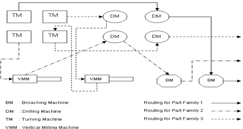
competitiveness in a dynamic environment. The unpredictability of demand and changes in product mix will not significantly affect the efficiency or the operation of a VCMS. A virtual cell is a logical grouping of machines that are not necessary to be transposed into physical proximity, in which virtual means something not physically existing as such, but made by software to appear to do so logically. The advantages of virtual cellular manufacturing systems are reduced setup time, reduced work-in-process inventory, lowered lead time, ability to absorb changes in product mix and routing flexibility.
Fig 1 Virtual Cellular Manufacturing System
1.2 Fuzzy Logic
Fuzzy logic, which was introduced by Zadeh (1965), has been applied to various industrial problems including production systems. The advantage of the fuzzy logic system approach is that it incorporates both numerical results from a previous solution or simulation and the scheduling expertise from experiences or observation, and it is easy to implement. Fuzzy set based optimization was first introduced by Bellman and Zadeh where they addressed the concept of decision making in a fuzzy environment. These concepts have been frequently used and applied by researchers. The first method for solving fuzzy linear programming problems was proposed by Zimmermann. Using Zadeh’s work, he interpreted fuzzy decision set as a collection of goals and constraints denoted the max-min model. In the fuzzy decision set proposed by Zimmermann, the best fuzzy decision is the union of the aggregated intersections of goals and constraints. Thus Bellman and Zadeh’s idea leads to a well known approach called the maximizing decision approach. The main goal of this approach is to find the best solution with the highest membership degree in the fuzzy decision set. The main aim of fuzzy programming is to find the best solution under imprecise information and/or vague resource capacities where uncertain constraints are satisfied to the maximum possible degree. Depending upon whether the imprecision appears in the objective function, a set of constraints and/or technological matrix, there is a variety of approaches for solving fuzzy programming problems. Fuzzy logic, one of the problem solving methodology to arrive at a definite conclusion based on imprecise input information. Because of the increasing variety of consumer goods and decreasing product life cycles, most manufacturing organizations encounter fluctuations in product mix and demand, known as turbulent conditions. In the fuzzy mathematical programming, the real solution is obtained through the application of mathematical programming tools, such as linear programming for finding the optimal solution. In this paper, two main parameters namely part demand and available machine capacity, are considered as fuzzy numbers. Here the dynamic and uncertain conditions are to be considered simultaneously.
1.3 Simulated Annealing Algorithm
analogous to the internal energy of the system in that state. The goal is to bring the system, from an arbitrary initial state, to a state with the minimum possible energy. At each step, the SA heuristic considers some neighbour s' of the current state s, and probabilistically decides between moving the system to state s' or staying in state s. The probabilities are chosen so that the system ultimately tends to move to states of lower energy. Typically this step is repeated until the system reaches a state that is good enough for the application, or until a given computation budget has been exhausted.
1.4 Rank Ordering Clustering Method:
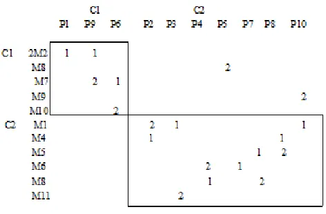
Rank Ordering clustering Technique facilitates the identification of part – machine clusters on the part machine incidence matrix. The rows and columns of 0’s and 1’s are considered binary numbers. The method repeatedly sorts rows and columns until no change occurs. Form groups of machines and part families in such a way that part families can be fully processed in a group of machines.
2. Literature review on VCMS:
Balakrishnan, J. and Cheng, C.H. (1996) presented a mathematical programming formulation for cellular manufacturing with changes in demand over time caused by product redesign and uncertainties due to volume variation, partmix variation and resource unreliability. Kannan et al. (1996) proposed a virtual cellular manufacturing approach for implementing cellular manufacturing systems that combines the set up efficiency obtained by traditional cellular manufacturing or group technology systems with the flexibility of a job shop. A virtual cell has been formulated that are temporary and logical in nature, allowing them to be more responsive to changes in demand patterns. Subash babu et al. (2000) proposed a new algorithm “Better alternative to ROC (BETROC)” which consists of distinct features to generate a number of alternative solutions. Mogaddam et al. (2005) proposed a nonlinear integer model of cell formation in dynamic condition and solved by some traditional metaheuristic methods such as genetic algorithm (GA), simulated annealing (SA) and tabu search (TS) and the results has been compared. Balakrishnan et al. (2005) generated a two stage procedure based on the generalized machine assignment problem and dynamic programming. One major characteristic of the proposed method was that the existing cell formation procedure has been flexible enough to incorporate. Cheng et a l. (2007) proposed a mathematical programming formulation for VCMS under multi-period planning horizon, with demand and resource uncertainties. Peng et al. (2007) presented a methodology to solve the manufacturing cell creation and the production scheduling problems for designing virtual cellular manufacturing systems (VCMS). The methodology consists of a mathematical model that describes the characteristics of a VCMS and includes constraints such as delivery due dates of products, maximum capacities of resources, critical tools limitation, and an ant colony optimization (ACO) algorithm for manufacturing cell formation and production scheduling. Nomden et al. (2008) conducted an extensive simulation study that: (1) a small number of alternative routes will mostly suffice, (2) a chained distribution of routes is preferable, and (3) additional secondary resources are relevant only under specific conditions. Saadettin et al. (2009) presented a multi-objective mixed integer programming formulation for job scheduling in virtual manufacturing cells (VMCs). In a VMC, machines has been dedicated to a part family as in a regular cell, but not physically relocated in a contiguous area. Kesen et al.(2009) proposed a multi objective mixed integer programming formulation for job scheduling in virtual manufacturing cells. The objective function has been designed to minimize the sum of makespan and total travelling distance/cost.
3. Literature review on Fuzzy Programming
Ozgur et al. (2007) developed the fuzzy programming model for cell formation based on machining times, utilization, workload, alternative routings, capacities, operation sequences. They also proposed the fuzzy programming model considering stochastic production requirements and alternative routes. Arikan, K and Gungor Z. (2007) developed a two phase procedure to solve multi objective fuzzy linear programming problems. They also proposed the interactive concept to reach simultaneous optimal solutions for all objective functions for different grades of precision according to the preferences of the decision maker (DM). Heng, Y.L. (2008) introduced the tolerance approach to solve semi infinite programming problem. He also used a quasi-newton line search using MATLAB software for implementation purpose. Mahdavi et al. (2008) proposed a fuzzy linear programming approach to minimize the total cost of inter cell and intra cell movements and the cost of machines. Considerations of uncertain conditions, batch material handling movements and sequence of operations has been considered as main advantage of the proposed model. Mehdi et al. (2009) applied the goal programming concept to minimize the deviation among the multiple costs of fuzzy flows and the given targets when the fuzzy supplies and demand are satisfied. Thakre et al. (2009) proposed a method for fuzzy linear programming problem with the help of multi objective constrained linear programming problem when the constraint matrix and the cost coefficients are fuzzy in nature.
4. Literature review on Simulated Annealing Algorithm
Harhalakis et al. (1990) applied simulated annealing algorithm for the manufacturing cell design problem which consists of designing cells of limited size in order to minimize inter-cell traffic and compared the results to the ones obtained using the so-called twofold heuristic algorithm. Boctor (1991) formulated a zero – one linear formulation for the cell formation problem and solved using simulated annealing algorithm to find the optimum solution upto 64.4% (solution for 58 out of 90 problems).Venugopal and Narendran (1992)developed an algorithm based on simulated annealing to solve the machine-component grouping problem for the design of cells in a manufacturing system. The proposed algorithm has been tested on sample problems and investigated for its sensitivity to some of the parameters and compared with K-means algorithm. Lee et al. (1992) developed a dual-objective simulated annealing approach for the purpose of concurrently forming machine cells and part families for cellular manufacturing in order to improve the performance of simulated annealing. Liu et al. (1993) introduced penalty costs into the objective functions to prevent the solution from violating the given constraints in the application of simulated annealing algorithm to machine cell formation problem. A near-optimal solution within a polynomial time even for the large-scale problems of machine cell formation has been obtained by using simulated annealing algorithm. Sofianopoulou (1997) proposed a mathematical model to minimize inter cell movement and to determine part movement and applied SA for solving manufacturing design with alternative process plans and/or replicate machines. Chen et al. (1998) developed a SA based heuristic applied to cell formation problems to minimize the number of inter cell movement for large size problems. Xambre et al. (2003) presented a mathematical model for the cell formation problem with multiple identical machines, which minimize the intercellular flow and solved using simulated annealing algorithm. ai Wu et al.(2008) proposed a simple yet effective simulated annealing-based approach, SACF, to solve the cell formation problem. He also provided considerable efforts to the design of parts and machine assignment procedures to direct SACF to converge to solutions with good values of grouping efficacy. Lin et al. (2009) proposed a simulated annealing-based meta-heuristic for solving part-machine cell formation problem (PMCFP) and compared the effectiveness of the proposed approach with conventional algorithms across a set of PMCFPs.
5. Literature review on Rank Order Clustering Method
6. Methodology
The methodology shown in figure1 describes the following. First is the formation of the mathematical model for virtual cellular manufacturing systems and second is the formation of four standard problems including two fuzzy parameters such as demand and the capacity .The four standard problems are shown in Table 1, which consists of four combinations of demand and capacity such as high demand and low resource, low demand and high resource, high demand and high resource and low demand and low resource. Third step is finding the upper and lower bound of the optimal solution for fuzzification According to the definition of lambda cut, the fuzzy demand can be expressed in terms of decision level λ as (1-λ) ) in which λ lies between 0 to1. The virtual cells are formed for optimal solution obtained from the maximizing decision level.
6.1 Mathematical Model
The following are the assumptions used in formation of mathematical model: 1. Each part type has a number of operations according to the known sequence.
2. The processing times for all operations of part types on different machines are known and deterministic.
3. The demand of each part type is given as a piecewise fuzzy number.
4. The capability of each machine type is known. Also the capacity of each machine in each period is given as a piecewise fuzzy number.
5. The fixed cost of each machine type is known.
6. The variable cost of each machine type is known. This cost indicates the operating cost that is dependent on the workload allocated to the machine.
7. Parts are moved among and within cells in batches.
8. The maximum number of cells must be specified in advance and it remains constant over time. 9. The upper bound of the cell size is known in advance.
10. Each machine type can perform one or more operations. Each operation can be done on different machine types with different processing times.(i.e, routing flexibility).
The proposed model is
min Z = ∑ ∑ ∑ + ∑ ∑ ∑ ∑ ∑
+ ∑ ∑ ∑ ∑ G ∑ ∑ …...(1) s.t
∑ ∑ 1 , , , ……….(2)
∑ ∑ , , , ………..(3)
∑ , , ………(4)
The first part in equation 1 represents the fixed cost of all machines required in all cells over the planning horizon. This cost is obtained by the product of the number of machine type m in cell c in period h and their associated costs. The second part in equation 1 is the variable cost of all machines required in all cells over the planning horizon. It is the sum of the product of the workload allocated to each machine type and their related costs. The third part in equation1 calculates the total logical group movement cost. It is the sum of the product of the number of logical movement between machines resulting from both consecutive operation of each part type and the cost of transferring of each part type between logic groups. Equation 2 guarantees that each part-operation is assigned to one machine and one cell at each period. Equation 3 is the fuzzy constraint of the model ensuring that the total available capacity of each machine in each cell satisfies as much as possible the assigned workload. Equation 4 ensures that the number of machines allocated to each cell does not violate the maximum cell size.
Input Parameters used in mathematical model are: H number of periods
P number of part types
C maximum number of cells can be formed in each period
fuzzy demand for part type p in period h
batch size for logic group movements of part type p G Logic group movement cost per batch
fixed cost of machine type m per period
β variable cost of machine type m for each unit time (1 hr)
fuzzy capacity of machine type m in terms of unit time in each period UB maximum cell size
time required to process operation j of part p on machine m
= 1 if operation j of part type p can be done on machine type m; otherwise 0 Decision variables used in mathematical model are:
=1 number of machine type m assigned to cell c at the beginning of period h ; otherwise 0.
=1 if operation j of part type p is performed in cell c in period h by machine type m; otherwise 0.
6.2 Fuzzification
Fuzzification is the process of transforming a crisp set to a fuzzy set, i.e., crisp quantities are converted into fuzzy quantities and can be represented by a membership function. The membership function, used to define a set and is denoted by the letter µ .Membership function defines the fuzziness in a fuzzy set and is generally represented by
μ (X) =
1 ∑ , ∑
∑ ; 0 ∑
…(5)
μ (X) is the degree to which solution X satisfying the fuzzy objective function. To define the membership function for the fuzzy constraint of the proposed model, the fuzzy mean workload assigned to each machine type m in cell c in period h, (X), with respect to the current solution X ,as follows:
: ∑ ∑ ≤ →
(X) = ∑ ∑ ≤ , c, h
The membership function for each fuzzy constraint of the proposed model is defined as
(X) =
0 if
∑
if ZL ∑ ; , … , … 6
1 if
Where =
∑ ∑
, =
∑ ∑
According to the concept of maximizing decision the fuzzy decision max λ
s.t :
λ ≤ μ X =
∑
6.3 Implementation of the developed fuzzy programming based approach The membership function of the optimal objective function values is
μ X
1 if Z X ,
, if Z X ,
0 if Z X ,
Where Z(X) includes fuzzy coefficients and
fuzzy capacity.
Four standard problems developed for the proposed model Min = Z ( )
s.t
∑ ∑ ≤ , ,
Min = Z ( ) s.t
∑ ∑ ≤ , ,
Min = Z ( ) s.t
∑ ∑ ≤ , ,
Min = Z ( ) s.t
∑ ∑ ≤ , ,
Let = min ( , , , ) and = max ( , , , ). 6.4 Defuzzification
Defuzzification is the process of converting fuzzy results into precise quantity by lambda- cut, where λ can be expressed in terms of decision level in which λ lies between 0 to 1.
According to Zadeh’s principle, the membership function of set D is defined by the intersection of sets G and Ci as D = G 1 2 … .
μ (X) = min { μ (X) , μ (X)}} μ (X) = membership function of set D
λ = ( μ (X) ) = (min μ X , μ X )……….(7) By maximizing decision method, Max λ such that
max
s.t constraints (2)-(4) and λ ( - - (∑ ∑ ∑ `
1
1 ;
1 1 , , . … … … 8
7. Data collection
The following data is collected from the manufacturing industry, which contains the machine details including fixed cost (alpha), variable cost (beta), logical group movement cost (Gamma) and plant capacity and part details including processing times, batch sizes and demand etc. The data set consists of twelve machines, ten parts and demand for time period of three months and the number of period as two. Ten different parts each consists of three operations are processed on these machines. The parts are produced according to operational sequences specified in their process sheet.
8. Computation results and Discussions
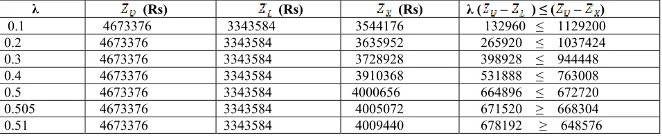
. From table, = max (4673376, 3343584, 4531536 and 3373152) = 4673376 and = min (4673376, 3343584, 4531536 and 3373152) =3343584. By using the maximizing decision level, the value for lambda is calculated such that it satisfies the condition λ( where is the calculated value for various values of lambda in equation 5 . Table 3 shows the calculations for finding the optimal value of lambda in equation 5. Table 4 shows the best solutions obtained from the maximizing decision problem and the optimal value of the decision level and objective function is obtained as λ =0.5 and Z(x) = 83347 $. The value of µ is calculated by = = = 0.5058. For example, with respect to the obtained optimal solution, the number of machine in cell 1 in period 2 is obtained as = 2 and = 1, = 1. In addition according to data set =0.56, = 0.57,
800, 400 =[400X (0.56+0.57)]/2 =226 =[800X (0.56+0.57)]/2 =452. Consequently, the
membership degree of X in the fuzzy set of constraint is (450 -226)/[(452-226) +34] =0.861. In other words X satisfies constraint with degree 0.861. According to equation (7), λ =0.5 is less than µ (X) = 0.5058 and µ (x)
= 0.861.
Table-1 Optimal solutions for the four standard problems (10 Parts,12 Machines)
Model no Zi (Rs) Machine fixed
cost (Rs) Machine variable cost (Rs)
Logical group movement cost (Rs)
CPU Time (h)
1 4673376 1684800 2679408 309168 0:29:14
2 3443584 1214880 1914288 214416 0:41:12
3 4531536 1614240 2609376 307920 0:36:14
4 3343584 1214880 1943338 214944 0:19:40
Table -2 Calculations to find max λ using maximizing decision level
λ (Rs) (Rs) (Rs) λ ( – ) ≤ ( – ) 0.1 4673376 3343584 3544176 132960 ≤ 1129200
0.2 4673376 3343584 3635952 265920 ≤ 1037424 0.3 4673376 3343584 3728928 398928 ≤ 944448 0.4 4673376 3343584 3910368 531888 ≤ 763008 0.5 4673376 3343584 4000656 664896 ≤ 672720 0.505 4673376 3343584 4005072 671520 ≥ 668304 0.51 4673376 3343584 4009440 678192 ≥ 648576
Table-3 Optimal solution obtained from the maximizing decision problem
λ Z(X)
(Rs) Machine fixed cost (Rs) Machine variable cost(Rs) Logical group movement cost(Rs) CPU Time (h)
0.5 4000656 1476480 2270736 262224 0:30:52
9. Cell formation
Fig. 2 The formed cells resulted from maximizing decision problem under decision level
λ = 0 .5(Period1)
Fig.3 The formed cells resulted from maximizing decision problem under decision level
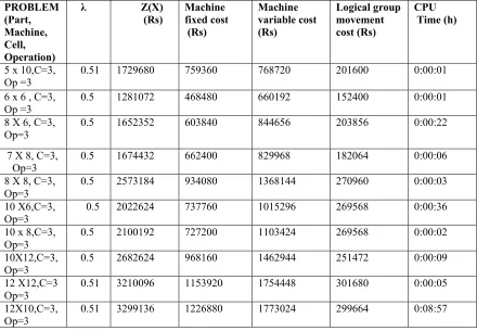
Table 4 Optimal solution obtained from the maximizing decision problem PROBLEM (Part, Machine, Cell, Operation)
λ Z(X) (Rs) Machine fixed cost (Rs) Machine variable cost (Rs) Logical group movement cost (Rs) CPU Time (h)
5 x 10,C=3,
Op =3 0.51 1729680 759360 768720 201600 0:00:01 6 x 6 , C=3,
Op =3
0.5 1281072 468480 660192 152400 0:00:01 8 X 6, C=3,
Op=3 0.5 1652352 603840 844656 203856 0:00:22 7 X 8, C=3,
Op=3
0.5 1674432 662400 829968 182064 0:00:06 8 X 8, C=3,
Op=3 0.5 2573184 934080 1368144 270960 0:00:03 10 X6,C=3,
Op=3 0.5 2022624 737760 1015296 269568 0:00:36 10 x 8,C=3,
Op=3 0.5 2100192 727200 1103424 269568 0:00:02 10X12,C=3,
Op=3
0.5 2682624 968160 1462944 251472 0:00:09 12 X12,C=3
Op=3 0.51 3210096 1153920 1754448 301680 0:00:05 12X10,C=3,
Op=3 0.51 3299136 1226880 1773024 299664 0:08:57
Table-5 Optimal solution and Cell formation obtained from the maximizing decision problem
PROBLEM SIZE (Part, M/c, Cell, Operation)
λ Z(X)
(Rs) Cell 1 Cell 2 Cell 3
Machine Parts Machine Parts Machine Parts
5x10,C=3
Op =3 0.51 1729680 M5,M7,M3 P1,P2 M2,M4, M10 P3,M6 M6,M8,M9 P4,P5 6 x 6,C=3
Op =3 0.5 1281072 M1,M2 P1,P2 M3,M4, M5 P4,P5 M3,M6 P3
8 X6,C=3
Op=3 0.5 1652352 M2,M5,M6 P4,P5 M1,M2, M3 P1,P2,P3,P6 M3,M4 P7,P8 7X8,C=3
Op=3 0.5 1674432 M6,M7,M8 P5,P1 M1,M2, M3,M4 P2,P3,P6 M1,M4,M5 P7,P4 8X8,C=3,
Op=3 0.5 2573184 M3,M4 M5,M6 P3,P4, P5 M1,M2, M3,M4, M7,M8
P1,P7 M2,M6,M8 P2,P6,P8
10X6,C=3 Op=3
0.5 2022624 M2,M3,M5 P3,P4 M1,M2, M4,M6 P1,P2,P5, P7,P9, P10 M1,M3, M4,M5 P6,P8 10X8,C=3
Op=3 0.5 2100192 M4,M7, M3,M8 P3,P6, P8 M1,M6, M2,M4 P1,P2,P5, P7,P9 M3,M5,M1 P9,P10, P4 10X12,C=3,
Op=3 0.5 2682624 M1,M7, M8,M9, M11
P7,P8 M2,M3, M4,M5, M6,M10
P1,P4,
12X12,C=3 Op=3
0.51 3210096 M1,M2,M8 M9,M10, M11
P2,P3, P1O,P11
M1,M3, M4,M5,M6 M10,M12
P1,P4,P5 P6,P8,P9
M2,M3, M7,M8
P12,P7
12X10,C=3
Op=3 0.51 3299136 M2,M4,M6 M8,M9, M10
P2,P5,
P8,P10 M1,M3,M4 M5,M6,M9 M10
P1,P4,P6 P9,P11, P12
M1,M2,M7
M7,M8 P3,P7
10. Comparative study
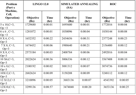
The comparison of the objective (total minimum costs) and the computation time for ten instances between Fuzzy Logic , Simulated Annealing algorithm (SA) and Rank Order clustering Algorithm (ROC) is shown in Table 6. Table 7 shows the difference in value of objective function between fuzzy logic, simulated annealing and rank order clustering algorithm. The results for objective and computation time between fuzzy logic using LINGO 12.0 and SA and ROC using C program are compared in table 8 and 9. The comparison graph for objective (total minimum costs) and computation time between LINGO 12.0, SA and ROC are shown in figure 4 and 5. The comparison of the objective (total minimum costs) between LINGO 12.0 and SA for period 2 and 3 are shown in table 10 and 11.The comparison graph for objective (total minimum costs) for period 2 and 3 between LINGO 12.0 and SA are shown in figure 6 and 7.The comparison of the logical group movement costs between LINGO 12.0 and SA for period 2 and 3 is shown in table 12 and 13. The comparison graph between logical group movement costs between LINGO 12.0 and SA for period 2 and 3 is shown in figure 8 and 9.
Table- 6 Comparison of fuzzy logic, simulated annealing algorithm and rank order clustering algorithm.
Problem LINGO 12.0 SIMULATED ANNEALING ROC
(Part x (SA)
Machine, Cell,
Operation) Objective Time Objective Time Objective Time (Rs) (hr) (Rs) (hr) (Rs) (hr)
5 x 10,C=3, Op =3
1729680 0:00:01 1695600 0:00:01 1772016 0:00:04 6 x 6 , C=3,
Op =3 1281072 0:00:01 1830096 0:00:04 1830144 0:00:08 8 X 6, C=3,
Op=3 1652352 0:00:22 2434656 0:00:31 2377248 0:00:23 7 X 8, C=3,
Op=3 1674432 0:00:06 1988640 0:00:21 2156400 0:00:12 8 X 8, C=3,
Op=3 2573184 0:00:03 2408784 0:00:06 2492016 0:00:04 10 X6,C=3,
Op=3
2022624 0:00:36 3006336 0:00:12 3567408 0:00:10 10 x 8,C=3,
Op=3 2100192 0:00:02 3081312 0:00:07 3074736 0:00:08 10X12,C=3,
Op=3 2682624 0:00:09 3158208 0:00:09 3248112 0:00:12 12 X12,C=3
Op=3
3210096 0:00:05 3683136 0:00:07 4543392 0:00:05 12X10,C=3,
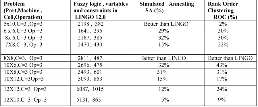
Table 7 The difference in value of objective function between fuzzy logic, simulated annealing and rank order clustering algorithm.
Problem (Part,Machine , Cell,Operation)
Fuzzy logic , variables and constraints in LINGO 12.0
Simulated Annealing SA (%)
Rank Order Clustering ROC (%) 5x10,C=3 ,Op=3 2198 , 382 Better than LINGO 2% 6 x 6,C=3 Op =3 1641, 295 29% 30% 8x 6,C=3 Op =3 2167, 385 32% 30% 7X8,C=3, Op=3
2470, 430 15% 22%
8X8,C=3, Op=3 2811, 487 Better than LINGO Better than LINGO 10X6,C=3 Op=3 2696, 475 32% 43% 10X8,C=3 Op=3 3493, 601 31% 31% 10X12,C=3Op=3 5093, 853 15% 17% 12X12,C=3 Op=3 6087, 1015 12% 24% 12X10,C=3 Op=3 5131, 865 5% 9%
Table 8 Comparison table for objective between LINGO 12.0, SA and ROC
Problem size
(parts, machines) LINGO 12.0 (Rs) SIMULATED ANNEALING (Rs) ROCA (Rs)
6,6 1,281,072 1830096 1830144
5,10 1729680 1695600 1772016
10,6 2377008 3006336 3567408
7,8 1674432 1988640 2156400
8,6 1652352 2434656 2377248
8,8 2573184 2408784 2492016
10,8 2100192 3081312 3074736
10,12 2682624 3158208 3248112
12,10 3299136 3474048 3653136
12,12 3210096 3683136 4543392
Fig 4 Comparison graph for objective between Lingo 12.0 , SA and ROC algorithm
0 1,000,000 2,000,000 3,000,000 4,000,000 5,000,000
0 2 4 6 8 10 12
fuzzy logic LINGO
SA (RS)
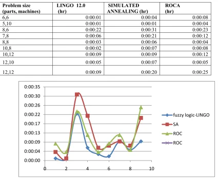
Table 9 Comparison table for computation time between LINGO 12.0, SA and ROC
Problem size (parts, machines)
LINGO 12.0 (hr)
SIMULATED ANNEALING (hr)
ROCA (hr)
6,6 0:00:01 0:00:04 0:00:08
5,10 0:00:01 0:00:01 0:00:04
8,6 0:00:22 0:00:31 0:00:23
7,8 0:00:06 0:00:21 0:00:12
8,8 0:00:03 0:00:06 0:00:04
10,8 0:00:02 0:00:07 0:00:08
10,12 0:00:09 0:00:09 0:00:12
12,10 0:00:05 0:00:07 0:00:05
12,12 0:00:09 0:00:20 0:00:25
Fig 5 Comparison graph for computation time between Lingo 12.0 , SA and ROC algorithm
Table 10 Comparison of objective between LINGO 12.0 and SA for period 2
Part , Machine Fuzzy Logic (LINGO 12.0) (Rs)
Simulated Annealing (SA) (Rs)
6,6 2369328 2875674
7,8 2977968 3756454
8,6 3119232 3956455
8,8 4000704 4956475
10,6 3720336 4268500
10,8 3917280 5465879
10,12 4898112 5978560
12,10 5860128 6378900
12,12 5500800 6167000
0:00:00 0:00:04 0:00:09 0:00:13 0:00:17 0:00:22 0:00:26 0:00:30 0:00:35
0 2 4 6 8 10
fuzzy logic‐LINGO
SA
ROC
Fig 6 comparison graph of Objective between LINGO 12.0 and Simulated Annealing (SA) for period 2
Table 11 Comparison of objective between LINGO 12.0 and SA for period 3
Part , Machine Fuzzy Logic (LINGO 12.0)
(Rs)
Simulated Annealing (SA)
(Rs)
6,6 3416160 3756760 7,8 4130736 5945654 8,6 4491504 6489365 8,8 5641824 6479500 10,6 5442432 7468320 10,8 5727504 9357465 10,12 7121952 8748645 12,10 7993248 10356780
Fig 7 comparison graph of Objective between LINGO 12.0 and Simulated Annealing (SA) for period 3 0
1000000 2000000 3000000 4000000 5000000 6000000 7000000
0 2 4 6 8 10
fuzzy logic LINGO (RS)
SA LINGO (RS)
0 2000000 4000000 6000000 8000000 10000000 12000000
0 2 4 6 8 10
Table 12 Comparison of Logical group movement cost between LINGO 12.0 and SA for period 2
Part , Machine Fuzzy Logic (LINGO 12.0)
(Rs)
Simulated Annealing (SA)
(Rs)
6,6 267648 266000 7,8 367632 562500 8,6 322464 263750 8,8 409488 562500 10,6 464160 972500 10,8 466560 821250
10,12 432336 512500
12,10 521856 564860
12,12 586012 855000
Fig 8 Comparison graph of Logical group movement cost between LINGO 12.0 and (SA) for period 2
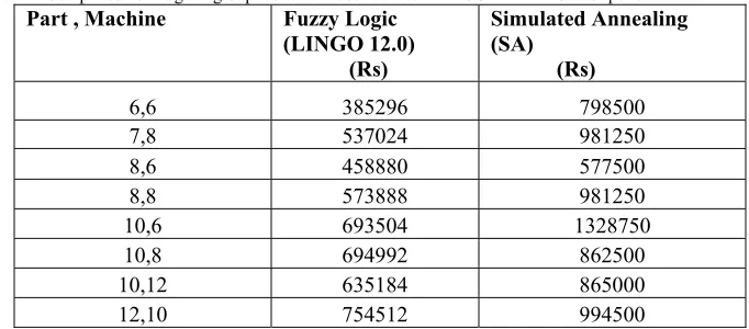
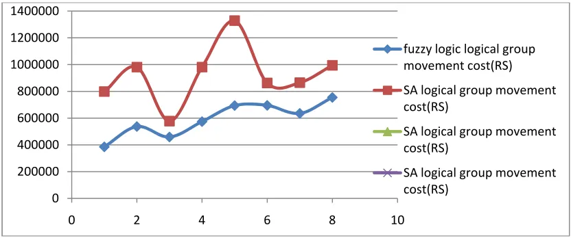
Table 13 Comparison of Logical group movement cost between LINGO 12.0 and SA for period 3
Part , Machine Fuzzy Logic (LINGO 12.0) (Rs)
Simulated Annealing (SA)
(Rs)
6,6 385296 798500
7,8 537024 981250
8,6 458880 577500
8,8 573888 981250
10,6 693504 1328750
10,8 694992 862500 10,12 635184 865000 12,10 754512 994500 0
200000 400000 600000 800000 1000000 1200000
0 2 4 6 8 10
fuzzy logic logical group movement cost(RS)
SA
Fig 9 Comparison graph of Logical group movement cost between LINGO 12.0 and Simulated Annealing (SA) for period 3
11. Conclusion
The mathematical model for the virtual cellular manufacturing system has been formulated and solved using optimization software LINGO 12.0.
Based on the results obtained in Table 3, the virtual cells has been formed for two periods.
The maximum difference in value of objective function between the simulated annealing algorithm, rank order clustering algorithm and fuzzy logic is 32 %( SA) and 43 %( ROC).
The minimum objective difference in value of objective function between the simulated annealing algorithm, rank order clustering algorithm and fuzzy logic. is 5 %( SA) and 2 %( ROC).
The difficulty of the developed fuzzy approach using Lingo 12.0 is to intensively increase in the computational efforts when the problem size increases.
The difficulty in fuzzy approach using LINGO 12.0 is the increase in computational efforts when the problem size increases.
12. Scope for future work
In the above work, the part demand and the plant capacity of the virtual cellular mathematical model are considered as fuzzy numbers. In future, the batch size are also considered as fuzzy numbers. In the present work, the logical group movement costs are considered as variables. In future, the logical group movement costs will also considered as fuzzy number. In the present work, the number of time period is considered as three and it may also increased further.
13. References
[1] King, J.R. (1980) ‘Machine-Component Grouping in Production Flow Analysis: An Approach using a Rank Order Clustering Algorithm’,
International Journal Of Production Research, Vol.18, No.2, pp.213 – 232.
[2] Chu, C.H. and Tsai, M. (1990) ‘A Comparison Of Three Array Based Clustering Techniques for Manufacturing Cell Formation’,
International Journal Of Production Research, Vol.28, No.8, pp.1417-1433.
[3] Harhalakis, G., Proth, J.M. and Xie, x.L.(1990) ‘Manufacturing Cell Design using Simulated Annealing: An Industrial Application’,
Journal Of Intelligent Manufacturing, Vol.18, No.2, pp.213-232.
[4] Boctor, F.F. (1991) ‘A Linear Formation of the Machine – Part Cell Formation Problem’, International Journal Of Production Research,
Vol.29, No.2, pp. 343-356.
[5] Lee, S. and Wang, H.P.(1992) ‘Manufacturing Cell Formation: A Dual – Objective Simulated Annealing Approach’, International Journal
Of Production Research, pp. 314- 320.
[6] Venugopal, V. and Narendran, T. (1992), ‘ Cell Formation in Manufacturing Systems through Simulated Annealing: An Experimental
Evaluation’, EuropeanJournal Of Operation Research, Vol.63,No.3, pp. 409-422.
[7] Liu, C.M. and Wu, J.K. (1993) ‘Machine Cell Formation : Using the Simulated Annealing Algorithm’,International Journal Of
Computer Integrated Manufacturing, Vol.6, No.6, pp.335 – 349.
[8] Kaparthi, S. and Suresh, N.C. (1994) ‘ Performance Of Selected Part –Machine Grouping Techniques for data sets of Wide Ranging Sizes
and Imperfection’, Decision Sciences, Vol.25, No.4, pp.515 – 539.
[9] Stefen, C. and Kuchta, D.(1996) ‘A Concept of the Optimal Solution of the Transportation Problem with Fuzzy Cost Coefficients’,
0 200000 400000 600000 800000 1000000 1200000 1400000
0 2 4 6 8 10
fuzzy logic logical group movement cost(RS)
SA logical group movement cost(RS)
SA logical group movement cost(RS)
[10] Narayanaswamy, P., Bector, C.R. and Rajamani, D. (1996) ‘Fuzzy Logic Concepts applied to Machine-Component Matrix formation in
Cellular Manufacturing’, European Journal Of Operation Research, pp.88-97.
[11] Slary, w. (1996) ‘Scheduling as a fuzzy multiple criteria optimization problem’, International Journal Of Fuzzy Sets and Systems,
pp.197-222.
[12] Kannan, V.R. and Ghosh, S. (1996) ‘Cellular manufacturing using virtual cells’, International Journal of Operations and Production
Management, Vol. 16, No. 5, pp. 99–112.
[13] Kannan, V.R. and Ghosh, S. (1996) ‘A virtual cellular manufacturing approach to batch production’, Decision Sciences, Vol. 27, No.3,
pp.519-539.
[14] Sofianopoulou, S. (1997), ‘Application of Simulated Annealing to a Linear Model for the Formulation of Machine Cells in Grouping
Technology’, International Journal Of Production Research,Vol.35, No.2, pp.501- 511.
[15] Chen, M. (1998), ‘A Mathematical Programming Model for Systems Reconfiguration in a Dynamic Cellular Manufacturing Environment’,
Annals Of Operation Research, Vol. 77, pp.109 – 128.
[16] Subash Babu, A., Nandurkar, K.N. and Austin Thomas. (2000) ‘Development of virtual cellular manufacturing systems for SMEs’,
International Journal of Logistics Information Management, Vol.13, No. 4, pp.228-242.
[17] Gasimov, R.N. and Yenilmez, K. (2002) ‘Solving fuzzy linear programming problems with linearmembership functions’, pp.375-396.
[18] Bijay, B.P. and Moitra, B.N.(2003) ‘ A Goal Programming Procedure for Solving Problems with Multiple Fuzzy Goals Using Dynamic
Programming’, European Journal Of Operation Research, pp.408- 491.
[19] Xambre, A.R. and Vilarinho, P.M. (2003) ‘A Simulated Annealing Approach for Manufacturing Cell Formation with Multiple Identical
Machines’, European Journal Of Operation Research, pp.434-446.
[20] Arikan, F. and Gungor, A. (2005) ‘A Parametric model for Cell formation and exceptional elements problems with fuzzy parameters’,
Journal of Intelligent Manufacturing, pp.103-114.
[21] Balakrishnan, J. and Cheng, C.H. (2005) ‘Dynamic Cellular Manufacturing under Multi-Period planning horizon, Journalof Manufacturing
Technology, pp.516-530.
[22] Moghaddam, R.T., Aryanezhad, M.B., Safaei, N. and Azaron, A. (2005) ‘Solving a dynamic cell formation using metaheuristics’,
International Journal of applied Mathematics and Computations, pp.761-780.
[23] Hachicha, W., Masmoudi, F. and Haddar, M. (2006) ‘ A Correlation Analysis approach Of Cell Formation in Cellular Manufacturing
System with incorporated production data’, International Journal Of Manufacturing Research, Vol. 1, No. 3, pp.332-353.
[24] Lu, Z., Ruan, D., Fengjie, W. and Zhang, G.(2007) ‘ An α –Fuzzy Goal Appropriate algorithm For solving fuzzy multiple Objective Linear
Programming Problems’, Journal of Soft Computing, pp.259- 267.
[25] Ozgur Eski and Ozkarahan, I. (2007) ‘A Simulation based Fuzzy goal Programming Model for Cell Formation’, International Conference
on fuzzy systems and Knowledge discovery, pp.305-312.
[26] Safaei, N., Saidi-Mehrabad, M., Moghaddam, R.T. and Sassani, F.(2007) ‘A fuzzy Programming approach for a cell formation problem
with dynamic and uncertain conditions’, International Conference of Computers and Industrial Engineering, pp.215-226.
[27] Arikan, F. and Gungor, G.(2007), ‘ A Two Phase Approach For Multi Objective Programming Problems with Fuzzy Coefficients’,
International Journal Of Information Sciences, pp. 5191-5202.
[28] Mak, K.L., Peng, P., Wang, X.X. and Lau, T.L. (2007) ‘An ant colony optimization algorithm for scheduling virtual cellular manufacturing
systems’, International Journal of Computer Integrated Manufacturing, Vol. 20, No. 6, pp. 524 – 537.
[29] Balakrishnan, J. and Cheng, C.H.(2007) ‘ Multiperiod Planning and Uncertainity Issues in Cellular Manufacturing : A Review and Future
Directions’, European Journal Of Operation Research, pp.281- 309.
[30] Heng, Y.L.(2008), ‘ An Approach for Solving Fuzzy Implicit Variational Inequalities with Linear Membership functions’, International
Journal Of Computers and Mathematics,pp.563-572.
[31] Mahdavi, I., Paydar, M.M., Heidarzade, A. and Amiri, N.M.(2008) ‘ Application of fuzzy mathematical approach for cell formation and
layout design with uncertain conditions’, Proceedings of the world congress on engineering, pp. 978-988.
[32] Nomden, G. and Van der Zee, D. (2008) ‘Virtual cellular manufacturing: Configuring routing flexibility’, International Journal of
Production Economics, Vol. 112, No.1, pp.439 – 451.
[33] Wu, T.H., Chang, C.C and Chung, S.H.(2008) ‘A Simulated Annealing Algorithm for Manufacturing Cell Formation Problems’,
InternationalJournal Of Expert Systems With applications, Vol. 34, No.3, pp.1609- 1617.
[34] Ghatee, M. and Mehdi Hashemi, S. (2009), ‘ Application of Fuzzy Minimum Cost Flow Problems to Network Design Under Uncertainity’,
International Journal Of Fuzzy Sets and Systems,pp.3263-3289.
[35] Saadettin, E.K., Sanchoy, K.D. and Gungor, Z.(2009) ‘ A Mixed Integer Programming Formulation For Scheduling Of Virtual
Manufacturing Cells(VCMS)’,International Journal Of Advance Manufacturing Technology, pp.--.
[36] Thakre, P.A., Shelar, D.S. and Thakre, S.P.(2009) ‘Solving fuzzy linear programming problem as multi objective linear programming
problem’, Proceedings Of World Congress On Engineering, pp. ---
[37] Kesen, S.E., Toksari, M.D., Zülal Güngör and Ertan Güner (2009) ‘Analyzing the behaviors of Virtual Cells (VCs) and traditional
manufacturing systems: Ant colony optimization (ACO)-based metamodels’, Computers and Operations Research archive, Vol. 36, No.7,
pp. 2275-2285.
[38] Lin, S.W., Ying, K.C. and Lee, Z.L. (2009) ‘Part- Machine Cell Formation in Group Technology Using a Simulated Annealing – based