JETIR1504085 Journal of Emerging Technologies and Innovative Research (JETIR) www.jetir.org 1297
PCA and FDA Based Dimensionality Reduction
Techniques for Effective Fault diagnosis of Rolling
Element Bearing
Vijay M Patil
1*,
Vishwash B
21Department of Mechanical Engineering, NMAMIT, Nitte, Udupi, India
Abstract— This paper uses Multi-Layer Perceptron Neural Network (MLPNN) for comparing the linear dimensionality reduction techniques (DRTs) for fault diagnosis in rolling element bearing (REB).The vibration signals from normal bearing (N), bearing with defect on ball (B), bearing with defect on inner race (IR) and bearing with defect on outer race (OR) have been acquired under different radial loads and shaft speeds. These signals were subjected to wavelet based denoising technique, from which 17 statistical features have been extracted. Linear DRTs namely, principal component analysis (PCA) and Fisher’s discriminant analysis (FDA) have been used to select the sensitive features. The selected features have been evaluated using MLPNN. Finally a comparison of Linear DRTs based on MLPNN performance is presented.
Keywords— Rolling element bearing, condition monitoring, Wavelet transform, PCA, FDA, MLPNN.
I.INTRODUCTION
Rolling element bearings (REBs) are one of the critical components in rotating machines and main driving devices in industrial machinery and equipment [1]. The majority of the failure arises from the defective bearings. Bearing failure leads to failure of a machine and unpredicted productivity loss for production facilities [2, 6]. Therefore condition monitoring of REB is very much essential to minimize machine down time, loss of production and to provide human safety. The traditional methods in this area involve noise analysis, temperature analysis, oil analysis and vibration analysis. Among these methods, vibration analysis is the most widely applied as it provides vital information about defects formed in the internal structure of the bearing [3].Common techniques used in vibration signal analysis are time and frequency domain analysis. Statistical information of the time domain signal can be used as trend parameters. They can provide information such as the energy level of the vibration signals and the shape of the amplitude probability distributions. High energy level of the vibration signals measured by the root mean square (RMS) values will indicate severely damaged components [5].
Noise present in the vibration signals degrades the quality of the features and will hide the features which contain valuable information about condition of the machine, therefore it is very much necessary to remove the noise from the acquired signals as much as possible. The features extracted from denoised signals gives best results when compared to the features extracted from raw vibration signals [5, 7]. Feature extraction is defined as a mapping process from the measured signal space to the feature space [10]. Feature extraction technique is essential for the effective fault diagnosis of bearing.
Usually signal data have high dimensionality in order to handle this data adequately, its dimensionality needs to be reduced. Dimensionality reduction is the transformation of high-dimensional data into a meaningful representation of reduced dimensionality [8]. Bearing defect detection is usually referred to as a classification problem. Artificial neural networks are information processing systems based on biological processing systems. Classifiers such as Artificial Neural Network (ANN), Adaptive Neuro-Fuzzy Interference System (ANFIS), and Support Vector Machines (SVM), have been used for bearing defect detection. [10].
This paper compares the performance of the linear DRTs (PCA, FDA). The vibration signals from Normal bearing (N), bearing with defect on ball (B), bearing with defect on inner race (IR) and bearing with defect on outer race (OR) have been acquired under variable loads and speeds conditions. These signals have been subjected to wavelet based denoising. The denoised signals have been decomposed using discrete wavelet transform (DWT) up to 4 level using Db4 mother wavelet. 17 statistical features have been extracted from 2nd level detailed wavelet coefficient (cd2) of non-overlapping vibration signals. Different DRTs as stated above have
been applied to downsize the feature dimension and select sensitive features. The best DRT has been selected based on MLPNN classifier performance results. Fig. 1 shows the proposed bearing fault diagnostic scheme used in this paper.
JETIR1504085 Journal of Emerging Technologies and Innovative Research (JETIR) www.jetir.org 1298
Fig 1. The proposed bearing fault diagnostic procedure.
II.DATAACQUISITION
Figure 2. Phographic view of the Test-rig of ball bearing available in Case Western Reserve University Bearing Data Center[14].
In this case study, the test data were acquired from the Case Western Reserve University Bearing Data Center [14]. As shown in Figure 2, the test-rig consists of a 2-horsepower motor (left), a torque transducer/encoder (center), a dynamometer (right), and control electronics. The test bearings support the motor shaft. Single point faults were introduced separately at the inner race, outer-race, and rolling element (i.e., ball) of the test bearing using electro-discharge machining with fault diameters of 7 mm. Faulted bearings were reinstalled into the test motor, and vibration data were recorded under different four states (normal, faults) using accelerometers, with motor loads of 3 horsepower, 0 horsepower and motor speeds of 1790 rpm, 1730rpm and a sampling frequency of 48,000 Hz.
III.DENOISING
JETIR1504085 Journal of Emerging Technologies and Innovative Research (JETIR) www.jetir.org 1299 for each level and reconstruction of the decomposed signal based on original approximate coefficients and modified detail coefficients .Daubechies wavelet of order 8 has been used as the mother wavelet for denoising the raw vibration signals which has been decomposed to 4 levels. Hard thresholding with universal threshold as threshold selection rule and multiplicative threshold rescaling has been done using level-dependent estimation of noise level which gave best denoised signal.
Figure 3. Sample plots for (a) raw signals (b) Wavelet based denoised
Vibration signals for the four bearing conditions: N, B, IR, and OR, at a speed of 1730 rpm and load of 3HP Load.
Fig 3(a). Shows raw vibration signals for four conditions of bearing and Fig 3(b). Shows corresponding denoised signals.
IV. FEATURE EXTRACTION
The denoised vibration signal data (250000 × 1) has been divided into 25 non-overlapping bins with each bin having 10000 data. Discrete wavelet decomposition is done up to 4 levels [5], which contains both approximate and detailed coefficients. Detail coefficients can then be used to reconstruct the original signal along with approximation coefficients by using Inverse Wavelet Transform (IWT).Seventeen statistical features have been extracted from the dominant wavelet coefficient (cD2).Statistical features extracted are given in table II.
TABLE II. STATISTICAL FEATURES. .
V. DIMENSIONALITYREDUCTIONTECHNIQUES
In this paper linear DRTs PCA and FDA have been applied and most prominent sensitive features have been selected out of the total feature set, resulting in the dimensionality reduction. The linear DRTs have been discussed below.
JETIR1504085 Journal of Emerging Technologies and Innovative Research (JETIR) www.jetir.org 1300 Principal component analysis (PCA) also known as the Karhunen–Loeve transform, is a basic method in the system of the multivariate analysis techniques. By transforming a complex data set to a simple one with lower dimension, PCA reduce the less significant information in data set for further computing. Because of its excellent capability in extracting relevant information from large data sets, PCA has been successfully applied in numerous areas including data compression, feature extraction, image processing, pattern recognition and process monitoring in recent years [1, 4].
The method of the PCA includes, computing the Eigen values of the covariance matrix obtained from the feature matrix. Only a few features, corresponding to those with high Eigen values have been considered for further analysis. Hence feature matrix has been reduced from high dimensionality to low dimensionality by neglecting unwanted features.
The PCA algorithm used in this paper is as follows:
1.Compute the mean feature vector,μ
𝜇 =1
𝑝∑ 𝑋𝑘 (1) 𝑝
𝑘=1
Where Xk is the kth pattern, (k=1 to p); p=number of patterns, X is the full feature set matrix.
2. Find the covariance matrix, C
𝐶 =1
𝑝∑{𝑋𝑘− μ} 𝑝
𝑘=1
{𝑋𝑘− μ}𝑇 (2)
Where, T represents matrix transposition
3. Compute Eigenvalues 𝜆𝑖
and Eigenvectors 𝜈
𝑖of covariance matrix (C)
(𝐶 − 𝜆𝑖𝐼)𝜈𝑖= 0 (3)
(i=1, 2, 3 ...q), q=number of features, where, I is a unit matrix
4. Estimating high-valued Eigenvectors
i) Arrange all the Eigenvalues
𝜆
𝑖 in descending order ii) Choose cumulative distribution rate (K)iii) No. of high valued
𝜆
𝑖can be chosen so as to satisfy below relationshipWhere, s = number of high valued Eigen values chosen
iv) Select Eigen vectors corresponding to highest Eigen values.
5. Extract reduced feature set matrix P (PCA feature set matrix) from full feature set matrix
P = 𝑉𝑇𝑋 (4)
Where, V is the matrix of selected Eigenvectors.
(B) Fisher discriminant analysis (FDA)
The FDA is an extension of the PCA. It depends on the mean and the standard deviations of the feature sets to compute the discriminant distance JkP,Q
the two classes P and Q [7]. FDA seeks to find a linear transformation that maximizes the between-class
scatter and minimizes the within-class scatter, in order to separate one class from others [9].The expression for computing the Fisher Discriminant Power (FDP) is given in equation (5).
𝐽𝐾𝑃,𝑄=
|𝑀𝑒𝑎𝑛(𝑡𝐾𝑃) − 𝑀𝑒𝑎𝑛(𝑡 𝐾𝑄)|2 [𝑆𝑡𝑑 (𝑡𝐾𝑃)]2+ [𝑆𝑡𝑑 (𝑡𝐾𝑄)]2
(5)
Where, JkP,Q is the Fisher discriminant distance between the two classes of REB, P and Q for the kth feature set; tkP and tkQ are
kth feature for the bearing conditions P and Q respectively (P and Q each may be the N bearing, bearing with the B defect , bearing
with the IR defect and bearing with the OR defect); Mean( ) and Std( ) are the mean and the standard deviation.
In this DRT six combination of classes have been considered. The discriminant distance for dual combinations of the bearing conditions have been calculated, i.e., JkN,,IR(for the N bearing and bearing with the IR defect), JkN,B(for N bearing and bearing with
the B defect) and JkN,OR(for the N bearing and bearing with the OR defect), JkIR,B(for the IR bearing and bearing with the B defect),
JETIR1504085 Journal of Emerging Technologies and Innovative Research (JETIR) www.jetir.org 1301 summations of the pair wise combinations of JkP,Q
are taken to estimate the FDP of a specific feature tk.Fig 4.shows the FDPs for
all the 17 features.
Fig 4. The FDPs for all the 17 features.
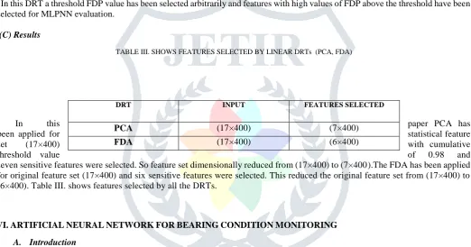
In this DRT a threshold FDP value has been selected arbitrarily and features with high values of FDP above the threshold have been selected for MLPNN evaluation.
(C) Results
TABLE III. SHOWS FEATURES SELECTED BY LINEAR DRTs (PCA, FDA)
In this paper PCA has
been applied for statistical feature
set (17×400) with cumulative
threshold value of 0.98 and
seven sensitive features were selected. So feature set dimensionally reduced from (17×400) to (7×400).The FDA has been applied for original feature set (17×400) and six sensitive features were selected. This reduced the original feature set from (17×400) to (6×400). Table III. shows features selected by all the DRTs.
VI.ARTIFICIALNEURALNETWORKFORBEARINGCONDITIONMONITORING
A. Introduction
ANN is a computational model that has one or more layers of processing elements called ‘neurons’. An ANN can be configured for a specific application, such as pattern recognition or data classification, through learning process [11]. Neural networks consists of many computing units called perceptrons which are arranged in layers and are interconnected. Each neuron is characterized by input, output, weight and an activation functions [10].
ANNs can be classified into two types: supervised learning neural networks and unsupervised learning neural networks. Supervised learning involves the presentation of both input and corresponding output patterns to the neural network during training [10]. The network learns all the patterns at the end of training and then the network is tested for its performance using patterns that are not used for training. Back Propagation (BP) algorithm is a powerful supervised learning algorithm. In unsupervised learning, only input patterns are presented to the network. The network learns the similarity in the input data, which will be obtained using any unsupervised learning algorithm [6, 7, 11].
The types of ANNs include multi-layer perceptron neural network (MLPNN), radial basis function (RBF) network, probabilistic neural networks (PNN).The most popular neural network is the MLPNN, which is a feed forward network and frequently exploited in fault diagnosis systems, which has found immense popularity in condition monitoring applications [6, 7].
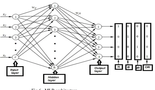
B) Multilayer Perceptron neural network (MLPNN)
MLPNN network consists of an input layer of source nodes, one or more hidden layers of computation nodes and an output layer. MLPNNs are a type of feed forward supervised learning neural networks and have been applied successfully to solve some difficult and diverse problems by training them with a popular algorithm known as Back-Propagation (BP) algorithm. This algorithm is based on the error-correction learning rule [12, 7].
The commonly used structure of the MLP neural network consists of three layers: input layer of source nodes, one or more hidden layer and an output layer. Fig. 6 shows the MLP architecture.
DRT INPUT FEATURES SELECTED
PCA (17×400) (7×400)
JETIR1504085 Journal of Emerging Technologies and Innovative Research (JETIR) www.jetir.org 1302
Fig 6. MLP architecture.
Each layer is comprised of nodes ≥ 1 and each node in any layer is connected to all the nodes in the neighboring layers. Input and output data dimensions of the ANN determine the number of nodes in the input and output layers respectively. The number of hidden layers and nodes in an MLPNN is proportional to its classification power. However, there is an optimum number of hidden layers and nodes for each case and considering more than those leads to over fitting of the classifier and substantially increases the computational cost and efforts [ 6, 7, 12].
C) Model Development
Statistical features extracted from the denoised vibration signals have been subjected to dimensionality reduction techniques like PCA and FDA to select few sensitive features which are used as inputs in the training and testing of the MLPNN. Only one hidden layer with different numbers of neurons 5, 10, 15, 20, 25, 30, 35, 40, 45 and 50 have been used in the hidden layer. A mean square error of 10-4, a minimum gradient of 10-10 and maximum number of epochs of 1000 has been used.
The patterns of the feature matrix are randomly mixed, out of which (80%) of them are used for training and the remaining (20%) have been used for testing the MLPNN. The number of nodes in the output layer is fixed to four, corresponding to the four conditions of the REB. A binary labelling scheme has been adopted for identifying the four conditions of the REB: N {1 0 0 0}, B{0 1 0 0}, IR{0 0 1 0} and OR{0 0 0 1}. The MLPNN trained with BP algorithm has been implemented by using the MATLAB Neural Network Toolbox [13].
VII. RESULTS AND DISCUSSION
The performance of MLPNN classifier for sensitive features selected using PCA and FDA are shown in table IV.
TABLEIV. PREDICTIONACCURACYONTESTDATA
The seven
features selected by PCA resulted in an accuracy of 76.50% on test data. The MLPNN performance increased for FDA with prediction accuracy of 89.75% due to different class considerations and PCA seeks to find the projection that maximize the total scatter across all classes whereas FDA tries to find discriminant projection that maximizes the between-class scatter and minimizes the within-class scatter effectively. Hence the FDA can be used as an effective DRT for fault diagnosis of bearing.
Table V. gives sample output results for FDA selected features for used in MLPNN with optimum simulation parameters.
TABLE V. SAMLPLE OUTPUT RESULTS FOR TEST DATA
DRT Training
Algorithm
Epochs No. of hidden Neurons
Error Accuracy on training data
(%)
Accuracy on test data (%)
PCA
BFG
1000
15
0.0021
93.75
76.50
FDA
BFG
1000
10
0.0017
98.50
89.75
Desired Output Network Output
N 1 0 0 0 0.99798 0.00954 -0.01055 0.00719
B 0 1 0 0 -0.1549 1.01254 0.01427 0.12271
IR 0 0 1 0 -0.01282 0.00047 1.04685 -0.00796
OR 0 0 0 1 -0.01399 0.05342 -0.00736 0.99927
JETIR1504085 Journal of Emerging Technologies and Innovative Research (JETIR) www.jetir.org 1303 VIII.CONCLUSION
In this paper an effort has been made to compare linear DRTs (PCA, FDA) based on ANN performance. The DRT is essential for achieving effective fault diagnostics and condition monitoring. FDA resulted in highest accuracy on test data with a dimension reduction in feature size for all load and speeds used in this work for condition monitoring of REB. MLPNN performance is highest FDA which is independent of load and speed condition, which is good for efficient fault diagnosis of REB.
ACKNOWLEDGMENT
We would like to thank the Case Western Reserve University Bearing Data Center (http://csegroups.case.edu/bearingdatacenter) for providing the bearing vibration signals data for carrying out the work presented in this paper and we would also like to thank Mr. Kumar H S for his necessary support and guidance.
R
EFERENCES[1] Kan Chen and Pan Fu, “The Feature Selection in Rolling Bearing Fault Diagnosis Based on Parts-Principle Component Analysis”, 2009 Fifth International Conference on Natural Computation, IEEE, pp. 613-616, 2009.
[2] Shaojiang Dong, Tianhong Luo, “Bearing Degradation Process Prediction Based on the PCA and Optimized LS-SVM Model”, Measurement,
vol.46, pp.3143–3152, 2013.
[3] Min Xia, Fanrang Kong, Fei Hu, “An Approach for Bearing Fault Diagnosis Based on PCA and Multiple Classifier Fusion”, IEEE, pp.321 -325, 2011.
[4] Xi Jianhui, Han Yanzhe and Su Ronghui, “New Fault Diagnosis Method for Rolling Bearing Based on PCA”, 25th Chinese Control and Decision Conference (CCDC), IEEE, pp. 4123 – 4127, 2013.
[5] Kumar H S, Dr. Srinivasa Pai P, Dr. Sriram N S and Vijay G S, “ANN Based Evaluation of Performance of Wavelet Transform for Condition Monitoring of Rolling Element Bearing”, International Conference On design and manufacturing, ICONDM, Procedia Engineering 64 ( 2013 ), pp. 805 – 814, 2013.
[6] Vijay GS, Srinivasa P Pai, NS Sriram, and Raj BKN Rao, “Radial Basis Function Neural Network Based Comparison of Dimensionality Reduction Techniques for Effective Bearing Diagnostics”, Journal of Engineering Tribology,Vol 227(6) ,pp 640–653, 2012.
[7] Vijay GS, “Vibration Signal Analysis for Defect Characterization of Rolling Element Bearing Using some Soft Computing Techniques”, Ph.D thesis, 2013.
[8] L.J.P. van der Maaten, E.O. Postma and H.J. van den Herik, “Dimensionality Reduction: A Comparative Review”, ELSEVIER, pp.186-194, 2008.
[9] Jinane, Claude delpha, Demba, “Linear Discriminant Analysis for the Discrimination of Faults in Bearing Balls by Using Spectral Features”,
First International Conference on Green Energy,IEEE , pp. 182-187,2014.
[10] C. Nataraj and Karthik Kappaganthu., " Vibration- based Diagnostics of Rolling Element Bearings: State of the Art and Challenges", 13th World Congress in Mechanism and Machine Science, Guanajua´to, Mexico, 2011.
[11] Abhinav Saxena and Ashraf Saad, “Evolving an Artificial Neural Network Classifier for Condition Monitoring of Rotating Mechanical Systems”, Applied Soft Computing 7, pp. 441–454, 2007.
[12] Dr. Jigar Patel et.al, “Fault Diagnostics of Rolling Bearing based on Improve Time and Frequency Domain Features Using Artificial Neural Networks”, International Journal for Scientific Research & Development,Vol. 1, Issue 4, pp.781-788,2013.
[13] MATLAB Neural Network Toolbox, Release R2012a.