190
Feature Selection Based On Hybrid Genetic
Algorithm With Support Vector Machine
(GA-SVM)
Waleed Dahea, H.S. Fadewar
Abstract: Curse dimensionality is the most problem in features fusion, data mining and pattern recognition. To solve this problem there are two methods:
Feature Reduction and Feature Selection (FS). In this paper, FS methods are analyzed from two side algorithms and data. FS is a very important task of selecting the most important subset of the feature with the minimum redundancy and the maximum relevant. In order to manipulate with the irrelevant features and redundant features in (high-medium-low) dimensional data, (high-medium-low) observations data and (binary classes, multiple classes) data. FS algorithms model based on the genetic algorithm with Support Vector Machine (SVM) as a fitness function is presented in this paper. Thus, our research tests experimentally how GA-SVM affects both the classification accuracy and the size of the feature subset for FS. GA-SVM is used to select the more significant features that obtain the optimum solution or nearest. Three different types of supervisor machine learning algorithms of classifiers are used in classification Naïve Bayes (NB), SVM and KNN. The performance of the proposed algorithm is tested on 11 UCI Machine Learning Repository data sets that belong to the University of California and is compared with other FS algorithms. Experiment results explain that the GA-SVM is efficient and can provide higher classification accuracy.
Index Terms: Genetic Algorithms, k-Nearest-Neighbor, SVM, Naïve Bayes, Classification, UCI Machine Learning Repository, Feature Selection, Feature
Reduction.
—————————— ——————————
1.
INTRODUCTION
Nowadays, An enormous number of different data is being gathered. Development of information technology growing fast, However, the data itself does not provide sufficient knowledge, and there are many unwanted or noisy data that should be identified. On the other hand, it will weaken decision-making. Feature selection (FS) is one of the most fundamental data preprocessing in data mining, pattern recognition and feature fusion. The purpose of FS is to select the optimal feature subset that contains the most valuable information for making better decisions. In addition, FS may work on a better comprehension of the domain, by maintaining only the features with a good understanding, corresponding to some importance criterion, to describe the essential patterns within the data and helps to reduce the effects of the curse of dimension [1]. We may estimate the optimal feature set according to maximize or minimize the function associated with the importance of the feature. FS is inherently a combinatorial optimization problem [1], [14]. It is a difficult task due mainly to the large search space, where the total number of possible solutions is 2n for a dataset with n features. There are available search strategies, such as complete search, greedy search, heuristic search, and random search. However, most existing feature selection methods suffer high time consumption and low recognition accuracy because of redundant and irrelevant features. Sometimes, it also leads to a local optimum. Therefore, constructing a model to reduce feature space effectively is integral.
Compared to the total feature space, the smaller feature space not only improves the computational speed but also provides a more compact model with better generalization capability. Mao and Tsang [2] proposed a two-layer cutting plane algorithm to search for the optimal feature subsets. Min et al. [3] developed a heuristic search and a backtracking algorithm to solve feature selection problems using rough set theory. The results show that the performance obtained by heuristic search techniques is similar to the backtracking algorithm. But the heuristic search cost less time. However, the papers barely mention the effect of decision structure information on the induced knowledge granules. Evolutionary computation (EC) techniques as effective methods have been applied to search for the optimal feature subset. Compared with popular search methods, the EC procedures do not need domain knowledge and do not make any presumption of the search space, for example whether it is linearly or nonlinearly separable, and differentiable [4]. Another important advantage of EC procedures is that their population-based mechanisms can produce various solutions on a single run. In the kinds of literature [5–7], Ant Colony Optimization (ACO), Particle Swarm Optimization (PSO) and Differential Evolution (DE) algorithm are adopted to optimize the feature space. Although the result may be sufficient for some tasks, the issue of unsettled still causes more time overhead. Therefore, with search space increasing, furthermore research on the stability of the algorithm is particularly significant. However, there is no search technology that will work well if the basic evaluation measure is poor. According to learning strategies, FS can be divided into supervised learning and unsupervised learning. In the former case, the class information is employed for choosing features; otherwise, one uses the distribution of a sample space to determine the possible hidden patterns. Based on the feature evaluation measure, FS can be classified into three categories: filters, wrappers and embedded methods [8]. The main difference is that wrapper approaches consist of a classification/learning algorithm to evaluate the goodness of the feature subset. For more attention paid to classification performance, wrapper algorithms are usually more time-consuming than filter algorithms. However, for a particular ————————————————
Waleed dahea
Research Scholar, School of Computational Sciences, SRTM University, Nanded, Maharashtra, India.
PH-7028798722.
E-MAIL: [email protected].
Dr. H.S. Fadware
Assistant Professor, School of Computational Sciences, SRTM University, Nanded, Maharashtra, India
191 classification algorithm, Wrappers usually perform better than
filters. However, filters have the advantage of lower-cost without considering classification accuracy. Finally, as for the embedded methods, a hybrid Fuzzy Min-Max-CART-Random Forest algorithm proposed by Seera and Lim [9] can be provided as a recent example. Chen et al. [10] proposed the CSMSVM method utilized a novel feature selection criteria, namely the margin verses cosine distance ratio, which adds the weight value of the features to maximize the margin verses cosine distance ratio. In an unsupervised scheme, the normalized mutual information score is employed for computing both the similarity and the dissimilarity in the literature [11]. A study by Brown et al. [12] also notes the good performance of the conditional mutual information maximization measure using the K-nearest neighbors (KNN) classifier. Although the search mechanism and evaluation criteria in the literature have improved the performance of the FS algorithm to a certain extent, the distribution of the data and the convergence of the algorithm have not been considered. Hongbin et at [13] notes that the feature selection problem is first studied from the perspective of sample granulation and feature granulation, and the novel hybrid genetic algorithm with granular information for feature selection and optimization is proposed. In this paper, in view of the advantage of global search ability, the improved GA-SVM is developed as the feature space search strategy. Each chromosome represents a solution from the perspective of the feature space, and the SVM is used to achieve fitness function of GA, and finally the optimized feature subset is obtained. The rest of the paper is organized as follows: In Section 2, related works on feature selection are reviewed, and the formal description of the genetic algorithm and the SVM is also discussed. Moreover, a detailed description of the proposed methodology is presented in Section 3. In Section 4, the experimental results and comparisons with other algorithms are given. Finally, the paper is summarized in Section 5.
2
2 RELATED
WORK
2.1 GENETIC ALGORITHM
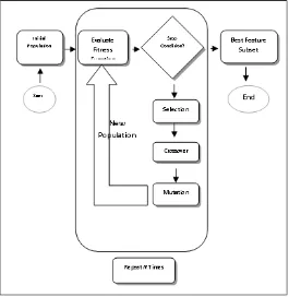
A Simple Genetic Algorithm (SGA) is a computational concept of biological evolution that can be used to solve optimization problems [15].These algorithms encode a potential solution to a particular problem on chromosome-like data structure and apply recombination operators to these structures so as to preserve significant information. An implementation of a genetic algorithm begins with a random population of chromosomes. One can evaluates these data structures and apply reproduction operators in such a way that the chromosomes which give a better solution to the objective problem are given more chances to reproduce themselves than those chromosomes which gives poorer solutions. The goodness of a solution is typically defined with respect to the current population. The formal description of the genetic algorithm is presented in this paper. The basic process of genetic algorithm is as follows: (1) initialization. Randomly generate N individuals as the initial population, and set the number of evolution as well; (2) individual evaluation. Calculate or evaluate the fitness of each individual according to the evaluation criteria; (3) population evolution. Employ the selection operation, the crossover operation and the mutation operation to produce the next generation; (4) termination test. If the maximum fitness of the individual is the optimal solution
or the maximum number of iterations, then terminate the calculation, otherwise return (2). SGA is illustrated in Figure 1.
2.2
SGA
OPERATORS
2.2.1 SELECTION
Chromosomes are selected from the current population to be parents to crossover. Based on Darwin’s evolution theory the best ones should survive and create new offspring. There are many methods to select the best chromosomes. They are Roulette Wheel selection, Boltzman selection, Tournament selection, Rank selection, Steady state selection and some other selection methods.
2.2.2 CROSSOVER
Crossover is a genetic operator that mates two chromosomes (parents) to produce a new chromosome (offspring). The idea behind crossover is that the offspring may be better than both of the parents if it takes the best characteristics from each of the parents. Crossover occurs during evolution corresponding to a user-definable crossover probability. Single point crossover, two-point crossover, Uniform crossover and Arithmetic crossover are the crossover method.
2.2.3 MUTATION
After crossover is performed, mutation takes place. This is to prevent falling all solutions in the population into a local optimum of solved problem. Mutation changes randomly the new offspring. For binary encoding a few randomly chosen bits are changed from 1 to 0 or 0 to 1. Here the selected bits are inverted.
2.2.4 EVALUATION
192 Figure 1: Simple Genetic Algorithm
2.3 CLASSIFICATION ALGORITHMS
2.3.1 K-NEAREST NEIGHBOR CLASSIFIER (KNN)
KNN is an instance-based classifier, which works on the assumption that classification of unknown instances can be identified by relating the unknown to the known instances according to some distance or similarity measure. The two instances far apart in the instance space defined by the appropriate distance function are less likely to belong to the same class than two closely situated instances. The KNN algorithm does not abstract any information from the training data during the learning phase. The process of generalization is postponed until the time of classification. Classification using a KNN classifier is done by locating the nearest neighbor in instance space and labeling the unknown instance with the same class label as that of the known neighbor. This approach is often referred to as a nearest neighbor classifier. The high degree of local sensitivity makes nearest neighbor classifiers highly prone to noise in the training data. The robust models can be achieved by identifying k, where k > 1, neighbors and the majority vote decide the outcome of the class labeling. If k=1, then the object is directly assigned to the class of its nearest neighbor. A higher value of k results in a softer, less locally sensitive function. To find the closeness normally some distance measures are used. Sometimes one minus correlation value is also taken as a distance metric. For continuous variables the following three distance measures are used. They are Euclidean distance, Manhattan distance and Minkowski distance. The Hamming distance must be used in the instance of categorical variables. In this work Euclidean distance is used as the distance measure.
2.3.2. SUPPORT VECTOR MACHINE CLASSIFIER (SVM)
SVM, a technique derived from statistical learning theory, is used to classify data points by assigning them to one of two disjoint half spaces [24]. They are able to classify non-linear relationships in the data through the use of kernel functions specific to the datasets. SVM is commonly used by many researchers in classification problems. It uses a nonlinear form to transform the original training data into a higher dimension. Within that new dimension it searches for the linear optimal separating hyperplane or a decision boundary separating the data of one class from another. The data from two different classes can always be separated by a hyperplane. The SVM finds the hyperplane with the help of support vectors and margins. SVM methods are much less prone to over fitting of data.
2.3.3. NAÏVE BAYES CLASSIFIER (NB)
NB is a classification technique based on Bayes’ Theorem with an assumption of independence among predictors. In simple terms, a NB classifier assumes that the presence of a specific feature in a class is unrelated to the presence of any other feature. NB model is simple to build and particularly useful for very large data sets. Along with simplicity, NB is known to outperform even highly sophisticated classification methods.
3.
P
ROPOSEDH
YBRIDG
ENETICA
LGORITHM WITHS
UPPORTV
ECTORM
ACHINE(GA-SVM)
3.1. CHROMOSOME REPRESENTATION
The chromosome should contain the information about the solution, which it represents. The most used way of encoding is a binary string. The random values are generated for gene position. The genes are considered when the value in its position is greater than 0.5, otherwise it is ignored. Figure. 2 shows the candidate solution representation(7 genes).
Figure.2 Chromosome Representation
3.2. FITNESS FUNCTION
The accuracy of SVM classifier is used as the fitness function for GA. The fitness function fitness(x) is defined as in (1).
fitness(x) =Accuracy(x) (1)
Accuracy(x) is the test accuracy of testing data x in the SVM classifier which is built with the feature subset selection of training data. The classification accuracy of SVM is given by (2).
Accuracy(x) = (c/t) X 100. (2) Where,
c - Samples that are classified correctly in test data by SVM technique
t - Total number of Samples in test data
3.3 K-FOLD CROSS VALIDATION
K-fold cross-validation is used for the result to be more valuable. In K-fold cross-validation, the original sample is divided into random K- subsamples; one among them is kept
g1 g2 g3 g4 g5 g6 g7
0.8 7
0.3 3
0.9 4
0.1 2
0.8 3
0.6 7
0.7 7
193 as the validation data for testing. The remaining1-K
sub-samples are used for training. The cross-validation process is repeated for k-times (the folds), with each of the K sub-samples used exactly once as the validation data. The average of k results from the folds gives the test accuracy of the algorithm. In order to achieve a reliable performance of the classifier, the 5-fold cross-validation method is used in this proposed method. Algorithm 1 shows the hybrid genetic algorithm with support vector machine.
ALGORITHM 1. HYBRID GENETIC ALGORITHM WITH SUPPORT VECTOR MACHINE
Input: S = (x1, x2, . . ., xn, y): Data set.
Where, x1,x2,..,xn are the features and y is the class Psize: Population number.
Csize: Chromosome length. Pc: Crossover probability. Pm: Mutation probability. T: Number of iterations.
Output: Best fitness and optimal feature subset OFS 1: Initialize algorithm parameters.
2: Load dataset S.
3: Sn =norm(S) // Normalizing the original data. 4: for i =1 to Psize do
5: for j =1 to Csize do
6: Pop(i, j) = round(rand) // Randomly initialize population.
7: end for(j) 8: end for(i)
9: for i =1 to Psize do
10: Subset = Sn(:, find(Pop(i, :) ==1)) 11: end for(i)
12: t = 0 // initialize iteration number.
13: While maximum number of iterations is not meet T 14: for i =1 to Psize do
15: Fitvalue(i) = fit1(pop(i)) //calculate fitness of individual by SVM.
16: sort(Fitvalue(i)) 17: end for(i)
18: Pop = Elit(pop) //elitist preservation is applied 19: Chrom(t,Pop)=Chrom(t,Popc)/crossover operation
20: Chrom(t, Popc) = Chrom(t, Popm) //mutation operation
21: NewPop = Pop //produce new population 22: t = t + 1
23: end While(13)
24: OFS = S(:, Find(Bestindividual(1, :) ==1))
25: return Best fitness and optimal feature subset OFS complexity of GA-SVM : (1) the time complexity of initializing population is O(Pr × Hr); (2) the time complexity of GA algorithm is O(m × q × nlogn), and the time complexity of training SVM classification is O(n × m) at least; (3) the time complexity of calculating fitness of individual is O(m × q × nlogn + n × m); (4) the sum of time complexity from crossover operator and mutation operator is O((Pr + Pc) × Hr). Thus, the time complexity of the GA-SVM is O(Pr × Hr) + O(T × Pr × (m × q × nlogn + n × m + (Pr + Pc) × Hr)) = O(Pr × (Hr + T × m × q × nlogn + T × n × m + T × Hr (Pr + Pc))).
Because q = m + z, where the z is a constant. Therefore, the time complexity of the algorithm is reduced to O (T × m × n × (mlogn + 1)) at least.
4.
EXPERIMENTAL
DESIGN
AND
RESULT
ANALYSIS
4.1 DATASET AND PARAMETER SETUP
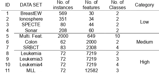
The used platform is Core i5-32430M @ 2.40 GHz, 6 GB RAM, and the simulations are implemented in Matlab R2019a. All the experiments are carried out by 10-fold cross validation method. For analyze the performance of the proposed algorithm from the perspective of features and samples respectively, the low, medium and high dimensional (Features) data sets are adopted in this paper. These data sets are available from the UCI machine learning repository or down loaded from the website: http://csse.szu.edu.cn/staff/zhuzx/Datasets. Hence, Table 1 tabulates the utilized data sets, including the number of features, the number of samples and the number of classes. In this section, we present several experimental studies about the GA-SVM on eleven datasets.
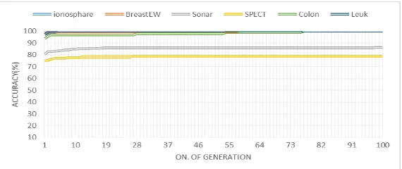
4.2 PERFORMANCE OF GA-SVM
In order to observe the performance of GA-SVM algorithm in each iteration process, the average accuracy curve of the 11
data sets in the 100 iteration are shown in Figure. 3. It can be seen from Figure. 3 that all the data sets accuracy obtained
Table 1. Description of used datasets.
optimal value smoothly by 100 iterations. Therefore, the algorithm can converge to the optimal value. In Figure. 3, some data sets show better performance, like Colon, MLL, Leukemia-3, Leukemia4, SRBCT and Ionosphere data sets, while the convergence of other data sets exist fluctuation. In this paper, the data sets are divided into two-class data sets figure.4, and multi-class data sets Figure5, to compare their accuracy speed and effect. It also shows that the GA-SVM algorithm can obtain the optimal value by iteration.
Table 2 shows the parameters of GA-SVM algorithm. ID DATA SET instances No. of features No. of Classes No. of Category
1 BreastEW 569 30 2
Low
2 Ionosphere 351 34 2
3 SPECTE 80 44 2
4 Sonar 208 60 2
5 Multi. Feat. 2000 649 10
Medium
6 Colon 62 2000 2
7 SRBCT 83 2308 4
8 Leukemia 72 7219 2
High
9 Leukemia3 72 7219 3
10 Leukemia4 72 7219 4
11 MLL 72 12582 3
GA Parameter Value
Chromosome Length No. of features
Population size 50
Crossover probability(Pc) 0.9 Mutation probability(Pm) 0.01
Number of Iteration 100
Fitness Function SVM
Crossover type Uniform
Mutation type Uniform
194 Table 2. GA-SVM parameters
Figure.3. The average accuracy value obtained by GA-SVM over its iteration for each dataset.
Figure. 4. The accuracy value of two-class data sets obtained by GA-SVM.
Figure. 5. The accuracy value of multi-class data sets obtained by GA-SVM.
Moreover, Table 3 reports the execution time of different methods for various data sets. In this paper, the BGA, mRMR [17], IBGAFG and INRSG algorithms are adopted to compare the time cost with the proposed method. As we can see in Table 3, the mRMR and INRSG algorithms runs less time in the low-dimensional datasets, but with the increase of dimension, the time cost increases rapidly. On high dimensional datasets, the IBGAFG and GA-SVM algorithms runs less time than the mRMR algorithm. In fact, both in low-dimensional and high low-dimensional datasets, a reduced set of
relevant and significant features is obtained using INRSG and GA-SVM algorithms with significantly lesser time.
Table 3. Execution time (in seconds) of different methods for various datasets.
A. EXPERIMENT ON LOW-DIMENSIONAL DATASET
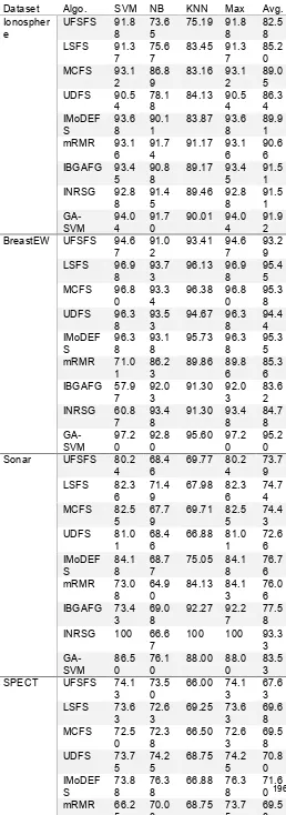
Table 4 compares the accuracy of various feature selection algorithms with the proposed algorithm GA-SVM on different classifiers. The results of the following algorithms are presented. (a) UFSFS [18] is the unsupervised feature selection that considering the feature similarity. (b) LSFS [19] is a feature selection method that based on Laplacian score. (c) MCFS [20] is the multi-cluster feature selection. (d) UDFS [19] is the unsupervised discriminative feature selection. (e) IMoDEFS [11] is the improved differential evolution. (f) mRMR [15] is the minimum Redundancy and Maximum Relevance algorithm for feature selection. (g) IBGAFG is the improved binary genetic algorithm with feature granulation for feature selection. (h) INRSG is the improved neighborhood rough set for feature selection. The proposed could explained the data as much as possible, that is to say, the classification performance of the proposed algorithms is superior than other algorithms. To evaluate the classification performance, the classification accuracy is compared with the results of the various well known and commonly used classifiers, such as Support Vector Machine (SVM), Naive Bayes (NB), IBk (KNN). Note that the Matlab 2019a software is used in the experimental analysis. In Table 4, the Max and Avg. present the maximum classification accuracy and average classification accuracy of three classifiers respectively. Table 4 shows the performance comparison of different feature selection algorithms on five low-dimensional and high-sample datasets. Each entry in the table includes the mean. By analyzing the experimental results, it is clear that IBGAFG, INRSG and GA-SVM return better classification accuracy. For example, in Ionosphere dataset, the GA-SVM achieves 94.04%, 91.70% and 90.01% classification accuracy on SVM, NB and KNN classifier respectively. The classification accuracy of GA-SVM is better than that of other algorithms on the three classifiers. The purpose of this section is just to test the improvement of classification accuracy.
B. EXPERIMENT ON MEDIUM AND HIGH-DIMENSIONAL DATASET In order to verify the performance of the proposed algorithm in the medium and high-dimensional dataset, this chapter adopts three evaluation criteria: the classification accuracy(ACC%), the number of feature(|S|) and the time cost(t(s)). Then, we compare proposed algorithm with the existing algorithms to prove the validity of the proposed algorithm. In Table 5, FCFB,
DATA SET BGA mRMR IBGAFG INRSG
GA-SVM*100
BreastEW 56.38 5.72 73.7 2.74 0.69
Ionosphere 389.65 5.36 472.63 13.32 0.71
SPECTE 25.34 5.42 29.43 3.00 0.68
Sonar 162.21 5.57 175.79 9.35 0.65
Multi. Feat. 8673.76 556.03 10414.51 12.83 22.79
Colon 66.82 1682.91 90.57 33.88 0.74
SRBCT 232.61 7.66 268.87 59.90 2.34
Leukemia 118.87 2083.56 605.22 109.77 0.97 Leukemia3 174.25 2865.87 698.69 107.28 1.87 Leukemia4 218.42 2490.57 616.49 108.27 2.94
195 BIRS, MBEGA, GA and mRMR five algorithms are compared
and analyzed. The FCFB [21] is a fast filtering method based on correlation. It selects a feature whose correlation coefficient is greater than a given threshold. The BIRS [22] is the wrapper method which based on the best incremental ranked subset according to some measure of interest. The MBEGA [23] is the Markov blanket-embedded genetic algorithm method, which based memetic operators add or delete features from a genetic algorithm solution so as to quickly improve the solution and fine tune the search. The GA [24] is the standard genetic algorithm that identifies suitable feature subsets solely based on the predictive ability of algorithm. The mRMR [15] is developed for feature selection based on mutual information, which maximize the correlation between features and class variables while minimizing the correlation between features and features. IBGAFG is the improved binary genetic algorithm with feature granulation for feature selection. INRSG is the improved neighborhood rough set for feature selection. Table 5 actually provides the information that how many the better features and how much better classification accuracy can be obtained by the proposed method. As can be seen from Table 5, although the dimension of the data set is quite high, GA-SVM can achieve 100% classification accuracy in one data sets: SRBCT. However, since the feature subset obtained by GA-SVM contains a large number of irrelevant or redundant features that makes the feature subset size still large. For example, in Leukemia, Leukemia-3, and SRBCT data sets, the number of features selected by the algorithm GA-SVM is 3582, 3604 and 1161.
Table 4. Performance comparison of different feature selection algorithms on high-observation and low-dimensional
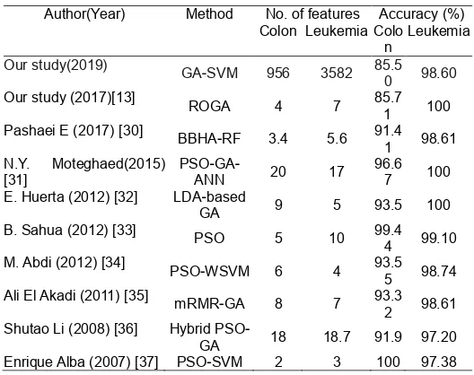
Author(Year) Method No. of features Accuracy (%) Colon Leukemia Colo
n
Leukemia
Our study(2019) GA-SVM 956 3582 85.5
0 98.60
Our study (2017)[13] ROGA 4 7 85.7 1 100 Pashaei E (2017) [30] BBHA-RF 3.4 5.6 91.4
1 98.61 N.Y. Moteghaed(2015)
[31]
PSO-GA-ANN 20 17
96.6 7 100 E. Huerta (2012) [32] LDA-based
GA 9 5 93.5 100
B. Sahua (2012) [33] PSO 5 10 99.4 4 99.10 M. Abdi (2012) [34] PSO-WSVM 6 4 93.5
5 98.74 Ali El Akadi (2011) [35] mRMR-GA 8 7 93.3
2 98.61 Shutao Li (2008) [36] Hybrid
INTERNATIONAL JOURNAL OF SCIENTIFIC & TECHNOLOGY RESEARCH VOLUME 8, ISSUE 12, DECEMBER 2019 ISSN 2277-8616
196 Table 5. Performance comparison of different feature selection
algorithms on medium and high-dimensional datasets
D at as et E va l Mea s. FC B F B IR S MB E GA GA mRMR IB G A FG IN R S G GA -S V M C olon ACC( %) 84.5 4 76.4 9 85.6 6
81.01 60.48 83.87 77.4 85.5
|S| 21.0 1.8 24.5 23.3 10.0 992 9 956 t(s) 1.1 56 70.6 66.8 1682.9
1 90.6 33.88 73.64
Le
uk
emi
a ACC( %) 93.8 2 89.3 4 95.8 9
92.31 61.81 100 98.6 1
98.6 0 |S| 32.8 2 12.8 25.2 10.0 3585 10 3582 t(s) 5.6 378.
2 112. 3
118 2083.5 6
605.2 109. 77 97.2 2 Le uk emi a-3 ACC( %) 95.7 6 84.4 9 96.6 4
90.96 54.17 100 97.2 2
97.2 5 |S| 77.7 2.4 18.1 75.1 10.0 3610 14 3604 t(s) 3.7 117
5.4 176. 6
174.2 2865.8 7
698.7 107. 28 187. 24 Le uk emi a -4 ACC( %) 92.3 8 77.6 0 91.9 3
88.06 47.92 93.06 91.6 7
93.3 0 |S| 99.3 2.2 26.2 74.4 10.0 3606 15 3638 t(s) 4.4 132
9.8 234. 3
218.4 2490.5 7
616.5 108. 27 294. 00 MLL ACC( %) 95.6 4 84.0 0 94.3 3
92.22 75.63 95.83 98.6 1
96.4 0 |S| 101.
6
3.7 32.1 75.4 10 6422 11 6218
t(s) 8.4 259 3.8
182. 1
165 74358 4.31 1203. 5 199. 52 241. 01 S R B C
T ACC(%) 98.94 86.66 99.23 95.77 95.59 100 98.80 100 |S| 98.6 4.1 60.7 78.4 10.0 1259 17 1161 t(s) 2.2 386.
8 246.2 232.6 7.66 268.9 233.75
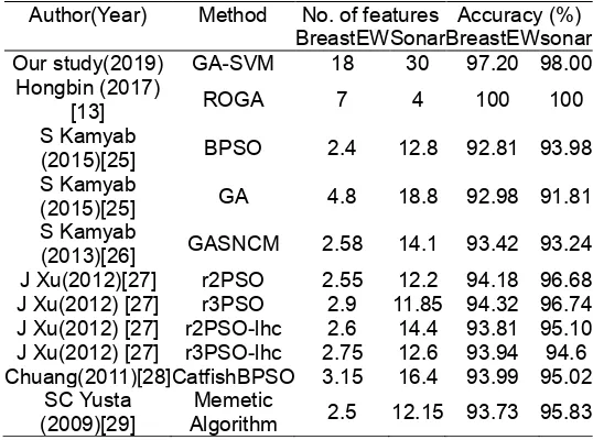
Comparison of our study with other studies in literature is an indispensable part to evaluate our proposed approach. On BreastEW and Sonar datasets, the experimental results of our method and the existing literatures are shown in Table 6. As can be seen, in Sonar dataset, the highest classification accuracy (100%) and the least features (4) are obtained with ROGA. While, the second highest classification accuracy (98.00%) and (30) feature subset obtained by our study, in BreastEW dataset, the classification accuracy is (97.20%) and feature subset is (18) are obtained by our study.
Table 6. Comparison the no. of feature and accuracy among the proposed methods and other approaches from literature in
BreastEW dataset and Sonar dataset.
In addition, Table 7 shows the selected features number and the classification accuracy obtained for Colon dataset and Leukemia dataset. As observed in Table 7, for Leukemia dataset, the classification accuracy achieved 98.60% and 3582 features are selected as the optimal feature subset. While for Colon dataset, the classification is 85.50% and 956 features are selected. Although less features are available, the proposed method may remove some important features that contribute to the improvement of classification accuracy. Based on the above analysis and comparison of previous work, our approach provides higher classification accuracy and smaller feature subset on some cases.
Dataset Algo. SVM NB KNN Max Avg.
Ionospher e
UFSFS 91.8 8
73.6 5
75.19 91.8 8
82.5 8
LSFS 91.3
7
75.6 7
83.45 91.3 7
85.2 0
MCFS 93.1
2
86.8 9
83.16 93.1 2
89.0 5
UDFS 90.5
4 78.18 84.13 90.54 86.34 IMoDEF
S 93.68 90.11 83.87 93.68 89.91
mRMR 93.1
6
91.7 4
91.17 93.1 6
90.6 6 IBGAFG 93.4
5
90.8 8
89.17 93.4 5
91.5 1 INRSG 92.8
8 91.45 89.46 92.88 91.51
GA-SVM 94.04 91.70 90.01 94.04 91.92 BreastEW UFSFS 94.6
7
91.0 2
93.41 94.6 7
93.2 9
LSFS 96.9
8 93.73 96.13 96.98 95.45
MCFS 96.8
0 93.34 96.38 96.80 95.38
UDFS 96.3
8 93.53 94.67 96.38 94.44 IMoDEF S 96.3 8 93.1 8
95.73 96.3 8
95.3 5
mRMR 71.0
1
86.2 3
89.86 89.8 6
85.3 6 IBGAFG 57.9
7 92.03 91.30 92.03 83.62 INRSG 60.8
7 93.48 91.30 93.48 84.78
GA-SVM 97.20 92.80 95.60 97.20 95.20
Sonar UFSFS 80.2
4 68.46 69.77 80.24 73.79
LSFS 82.3
6 71.49 67.98 82.36 74.74
MCFS 82.5
5 67.79 69.71 82.55 74.43
UDFS 81.0
1 68.46 66.88 81.01 72.66 IMoDEF S 84.1 8 68.7 7
75.05 84.1 8
76.7 6
mRMR 73.0
8 64.90 84.13 84.13 76.06 IBGAFG 73.4
3
69.0 8
92.27 92.2 7
77.5 8
INRSG 100 66.6
7 100 100 93.33 GA-SVM 86.5 0 76.1 0
88.00 88.0 0
83.5 3
SPECT UFSFS 74.1
3 73.50 66.00 74.13 67.63
LSFS 73.6
3 72.63 69.25 73.63 69.68
MCFS 72.5
0
72.3 8
66.50 72.6 3
69.5 8
UDFS 73.7
5 74.25 68.75 74.25 70.80 IMoDEF
197 Table 7. Comparison the no. of feature and accuracy among
the proposed methods and other approaches from literature in Colon dataset and Leukemia dataset.
5.
CONCLUSION
In this paper, the feature selection model based on hybrid Genetic Algorithm and Support Vector Machine (GA-SVM) is presented, the algorithm has strong robustness. Relying on our experimental results, the characteristics of our approaches are as follows: first, evaluate fitness value based on SVM, second, selecting smaller feature subset along with higher accuracy to be in next generation ; third, the rest are sent to crossover and mutation operations. Fourth and the most important, it proving successful for combining SVM and evolutionary algorithm and aggregating them into feature section for large-scale data. The proposed method is able to keep a good balance on the feature subset size and classification accuracy, which makes it more suitable for application areas such as pattern recognition and bioinformatics for biomarker discovery. In the further work, we plan to explore new search strategy and another method to improve the efficiency of the algorithm. Also, transforming feature selection into multi-objective optimization problem could be treated as a research subject in the future.
REFERENCES
[1] N. Spolaor, A.C. Lorena, H.D. Lee, Multi-objective genetic algorithm evaluation in feature selection, International Conference on Evolutionary Multi-Criterion Optimization (2011) 462–476.
[2] Q. Mao, W.H. Tsang, A feature selection method for multivariate performance measures, IEEE Trans. Pattern Anal. Mach. Intell. 35 (9) (2013) 2051–2063. [3] M. Fan, Q. Hu, W. Zhu, Feature selection with test
cost constraint, Int. J.
[4] Approx. Reason. 55 (1) (2014) 167–179.
[5] B. Xue, M. Zhang, W.N. Browne, X. Yao, A survey on evolutionary computation approaches to feature selection, IEEE Trans. Evolut. Comput. 20 (4) (2016) 606–626.
[6] S. Kashef, H. Nezamabadi-Pour, An advanced aco algorithm for feature subset selection, Neurocomputing 147 (2015) 271–279.
[7] K. Chakravarty, D. Das, A. Sinha, A. Konar, Feature Selection by Differential Evolution Algorithm – A Case Study in Personnel Identification, 2013.
[8] D.Y. Harvey, M.D. Todd, Automated feature design for numeric sequence classification by genetic programming, IEEE Trans. Evolut. Comput. 19 (4) (2014) 474–489.
[9] G. Gunday, G. Ulusoy, K. Kilic, L. Alpkan, Effects of innovation types on firm performance, Int. J. Prod. Econ. 133 (2) (2011) 662–676.
[10]M. Seera, C.P. Lim, A hybrid intelligent system for medical data classification, Expert Syst. Appl. 41 (5) (2014) 2239–2249.
[11]G. Chen, J. Chen, A Novel Wrapper Method for Feature Selection and its Applications, Elsevier Science Publishers B. V., 2015.
[12]T. Bhadra, S. Bandyopadhyay, Unsupervised feature selection using an improved version of differential evolution, Expert Syst. Appl. 42 (8) (2015) 4042–4053. [13]G. Brown, A. Pocock, M.J. Zhao, M. Lujn, Conditional likelihood maximisation: a unifying framework for information theoretic feature selection, J. Mach.Learn. Res. 13 (1) (2012) 27–66.
[14]Hongbin Dong, Tao Li∗, Rui Ding, Jing Sun, "A novel hybrid genetic algorithm with granular information for feature selection and optimization." Applied Soft Computing 65 (2018): 33-46.
[15]Dahea, Waleed, and H. S. Fadewar. "Multimodal biometric system: A review." International Journal of Research in Advanced Engineering and Technology, 4(1) (2018) 25-31.
[16]D.E. Goldberg, Genetic Algorithms-in Search, Optimization and Machine Learning. London: Addison-Wesley Publishing Company Inc, 1989.
[17]C. Cortes and V. Vapnik, ―Support-vector networks,‖ Mach Learn, 20( 3) (1995) 273–297.
[18]H. Peng, F. Long, C. Ding, Feature selection based on mutual information: criteria of dependency, max-relevance, and min-redundancy, IEEE Trans.Pattern Anal. Mach. Intell. 27 (8) (2005) 1226–1238.
[19]P. Mitra, C.A. Murthy, S.K. Pal, Unsupervised feature selection using feature similarity, IEEE Trans. Pattern Anal. Mach. Intell. 24 (3) (2002) 301–312.
[20]X. He, D. Cai, P. Niyogi, Laplacian score for feature selection, International Conference on Neural Information Processing Systems (2005) 507–514. [21]D. Cai, C. Zhang, X. He, Unsupervised feature
selection for multi-cluster data, ACM SIGKDD International Conference on Knowledge Discovery and Data Mining (2010) 333–342.
[22]L. Yu, H. Liu, Efficient feature selection via analysis of relevance and redundancy, J. Mach. Learn. Res. 5 (12) (2004) 1205–1224.
[23]R. Ruiz, Incremental wrapper-based gene selection from microarray data for cancer classification, Pattern Recogn. 39 (12) (2006) 2383–2392.
[24]Z. Zhu, Y.S. Ong, M. Dash, Markov blanket-embedded genetic algorithm for gene selection, Pattern Recogn. 40 (11) (2007) 3236–3248.
[25]M. Wahde, Z. Szallasi, A survey of methods for classification of gene expression data using evolutionary algorithms, Expert Rev. Mol. Diagnost. 6 (1) (2006) 101.
Author(Year) Method No. of features Accuracy (%) BreastEW Sonar BreastEW sonar Our study(2019) GA-SVM 18 30 97.20 98.00
Hongbin (2017)
[13] ROGA 7 4 100 100
S Kamyab
(2015)[25] BPSO 2.4 12.8 92.81 93.98 S Kamyab
(2015)[25] GA 4.8 18.8 92.98 91.81
S Kamyab
(2013)[26] GASNCM 2.58 14.1 93.42 93.24 J Xu(2012)[27] r2PSO 2.55 12.2 94.18 96.68 J Xu(2012) [27] r3PSO 2.9 11.85 94.32 96.74 J Xu(2012) [27] r2PSO-lhc 2.6 14.4 93.81 95.10 J Xu(2012) [27] r3PSO-lhc 2.75 12.6 93.94 94.6 Chuang(2011)[28] CatfishBPSO 3.15 16.4 93.99 95.02
SC Yusta
198 [26]S. Kamyab, M. Eftekhari, Feature Selection Using
Multimodal Optimization Techniques, Elsevier Science Publishers B.V., 2016.
[27]S. Kamyab, M. Eftekhari, Using a self-adaptive neighborhood scheme with crowding replacement memory in genetic algorithm for multimodal optimization, Swarm Evolut. Comput. 12 (2013) 1–17. [28]J. Xu, Y. Yin, H. Man, H. He, Feature selection based
on sparse imputation, International Joint Conference on Neural Networks (2012) 1–7.
[29]L.Y. Chuang, S.W. Tsai, C.H. Yang, Improved binary particle swarm optimization using catfish effect for feature selection, Expert Syst. Appl. 38 (10) (2011) 12699–12707.
[30]S.C. Yusta, Different metaheuristic strategies to solve the feature selection problem, Pattern Recogn. Lett. 30 (5) (2009) 525–534.
[31]E. Pashaei, N. Aydin, Binary black hole algorithm for feature selection and classification on biological data, Appl. Soft Comput. (2017).
[32]N.Y. Moteghaed, K. Maghooli, S. Pirhadi, M. Garshasbi, Biomarker discovery based on hybrid optimization algorithm and artificial neural networks on
microarray data for cancer classification, J. Med. Signals Sens. 5 (2) (2015) 88.
[33]E.B. Huerta, B. Duval, J.K. Hao, Gene selection for microarray data by a lda-based genetic algorithm, IAPR International Conference on Pattern Recognition in Bioinformatics (2008) 250–261.
[34]B. Sahu, D. Mishra, A novel feature selection algorithm using particle swarm optimization for cancer microarray data, Procedia Eng. 38 (5) (2012) 27–31. [35]Briefly, A novel weighted support vector machine
based on particle swarm optimization for gene selection and tumor classification, Comput. Math. [36]Methods Med. 2012 (9) (2012) 320698.
[37]A.E. Akadi, A. Amine, A.E. Ouardighi, D. Aboutajdine, A two-stage gene selection scheme utilizing mrmr filter and ga wrapper, Knowl. Inf. Syst. 26 (3) (2011) 487– 500.
[38]S. Li, X. Wu, M. Tan, Gene selection using hybrid particle swarm optimization and genetic algorithm, Soft Comput. 12 (11) (2008) 1039–1048.