Web: http://www.rothamsted.ac.uk/
Rothamsted Research is a Company Limited by Guarantee Registered Office: as above. Registered in England No. 2393175. Registered Charity No. 802038. VAT No. 197 4201 51. Founded in 1843 by John Bennet Lawes.
Rothamsted Repository Download
A - Papers appearing in refereed journals
Hassall, K. L. and Mead, A. 2018. Beyond the one-way ANOVA for
'omics data. BMC Bioinformatics. 19 (Suppl 7), p. 199.
The publisher's version can be accessed at:
•
https://dx.doi.org/10.1186/s12859-018-2173-7
The output can be accessed at:
https://repository.rothamsted.ac.uk/item/84664
.
© 9 July 2018. Licensed under the Creative Commons CC BY.
R E S E A R C H
Open Access
Beyond the one-way ANOVA for ’omics
data
Kirsty L. Hassall
*and Andrew Mead
From12th and 13th International Meeting on Computational Intelligence Methods for Bioinformatics and Biostatistics (CIBB 2015/16) Naples, Italy and Stirling, UK. 10-12 September 2015, 1-3 September 2016
Abstract
Background: With ever increasing accessibility to high throughput technologies, more complex treatment
structures can be assessed in a variety of ’omics applications. This adds an extra layer of complexity to the analysis and interpretation, in particular when inferential univariate methods are applied en masse. It is well-known that mass univariate testing suffers from multiplicity issues and although this has been well documented for simple comparative tests, few approaches have focussed on more complex explanatory structures.
Results: Two frameworks are introduced incorporating corrections for multiplicity whilst maintaining appropriate structure in the explanatory variables. Within this paradigm, a choice has to be made as to whether multiplicity corrections should be applied to the saturated model, putting emphasis on controlling the rate of false positives, or to the predictive model, where emphasis is on model selection. This choice has implications for both the ranking and selection of the response variables identified as differentially expressed. The theoretical difference is demonstrated between the two approaches along with an empirical study of lipid composition inArabidopsisunder differing levels of salt stress.
Conclusions: Multiplicity corrections have an inherent weakness when the full explanatory structure is not properly incorporated. Although a unifying ‘single best’ recommendation is not provided, two reasonable alternatives are provided and the applicability of these approaches is discussed for different scenarios where the aims of analysis will differ. The key result is that the point at which multiplicity is incorporated into the analysis will fundamentally change the interpretation of the results, and the choice of approach should therefore be driven by the specific aims of the experiment.
Keywords: Multiplicity, Model selection, ’omics, ANOVA
Background
Multivariate data are frequently generated within bio-logical applications due to the ever increasing availabil-ity of high-throughput technologies to study functional genomics using transcriptomics, proteomics, lipidomics and metabolomics. These technologies generate data from large numbers of response variables, and typically inter-est is focussed on identifying the ‘important’ response variables, where important will be a context specific def-inition. For instance, experiments may be designed with
*Correspondence:[email protected]
Computational and Analytical Sciences, Rothamsted Research, Harpenden AL5 2JQ, UK
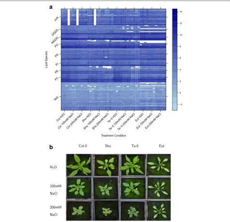
a specific explanatory structure, such as the inclusion of treatment factors, blocking factors or observational covariates, where important variables might be those for which different (combinations of ) treatment levels show statistically significant different responses. It is indis-putable that this explanatory structure information should be incorporated into the subsequent statistical analysis. However, this is not always straightforward to achieve. This is exemplified in a study of the lipid composition of
lipids (response variables) was measured in each condi-tion. The log2 abundance over these conditions for the
different lipid species is shown in Fig.1a. Interest might be focussed on lipids showing significant differences between different genotypes, salt stresses or combinations of these. There are two main avenues of analytical methods that can be applied to such ’omics data; multivariate methods and mass univariate methods (see e.g. [1,2]). Each have their own advantages and disadvantages, but in combina-tion can elicit a great deal of insight into the underlying mechanisms that generated the data [3–7]. In this paper,
we predominantly focus on the issues that arise in the lat-ter methods, the mass-univariate approach, but would like to emphasise that these methods should add to the insight obtained from multivariate approaches rather than act as a replacement.
Mass univariate analysis
In contrast to multivariate approaches, mass univari-ate methods investigunivari-ate each response variable inde-pendently. Although the covariance structure between response variables is not accounted for in such an analysis,
a
b
this approach will provide information about the vari-ability in individual response variables, and, in particular, how it relates to components of the explanatory structure. For example, identifying the sets of treatment conditions that are statistically significant for each response. This is particularly advantageous when an experiment may include complex explanatory structures that include mul-tiple explanatory terms. Standard statistical techniques such as ANOVA (analysis of variance), REML (restricted maximum likelihood) and regression can be used to inves-tigate both the biological size and statistical significance of different explanatory model components in an inferential framework. Moreover, these analysis approaches can cope with complex treatment structures (such as the factorial treatment structure in the above example), unbalanced design structures and missing values.
In generality, it is of interest to fit and analyse the following linear model,
yi=Xiβ+i, fori=1, ...,n (1)
i∼N(0,σ2),
wherenis the number of observations,yiis theith obser-vation of a single response variabley,Xiis theith row of the design matrixX,β is the vector of coefficients to be estimated and are independent error terms. Fitting and analysing such models is a completely standard statistical approach using the methods identified above.
However, there are issues in applying such methods en masse to many different response variables in the same dataset. To illustrate this, let us first consider the sim-ple examsim-ple where the design matrixXcorresponds to a single explanatory factor. Specifically, suppose
yji=βj+ji, i=1, ...,nj, j=1, ...,J (2) where yji is the ith observation on the jth treatment. Once fitted, the estimated parameters of this model can be assessed. Specifically, using either a two-sample t-test (forJ = 2) or an F-test (for J > 2) the null hypothesis of no difference in response in theJdifferent treatments can be tested. When testing at a pre-specified significance level, α, of 0.05, the probability of a type I error (the false positive rate) is controlled at 5%. However, it is well known that applying such a univariate analysis approach, en masse, to multiple response variables, will result in an unacceptably high type I error rate over the whole exper-iment due to the issue of multiple testing (also referred to as multiplicity), described below.
Multiple testing
In a multiple testing scenario, the probability of a type I error, or false positive (i.e. the probability of reject-ing the null hypothesis when the null hypothesis is true) over the tests for the complete set of response variables is inflated. For example, consider making independent
hypothesis tests for 10 (independent) response variables, the probability of making at least one type I error,α∗, is given by,
α∗=Prob(at least 1 type I error)
=1−Prob(no type I error)
=1−(1−α)10,
which when the individual level of significance is α = 0.05, givesα∗ = 0.40. Thus, to control the overall proba-bility overRtests (the number of response variables) of at least one type I error at a specified levelα, the significance level for each test becomes 1−(1−α)1/R, which in prac-tice is often approximated by the upper boundα/R, the Bonferroni correction. This adjustment controls the fam-ily wise error rate (FWER), defined to be the probability of at least one type I error. Alternative ways of controlling the type I error in a multiplicity framework include con-trolling the per-family error rate (PFER), which is defined to be the expected number of type I errors, and the false discovery rate (FDR), defined as the expected proportion of false discoveries. A plethora of methods for controlling the type I error, through differing multiple testing correc-tions, can be found in the literature (see [8,9] and [10] for reviews). These often have different aims, such as which error rate is to be controlled, whether or not tests can be considered independent and whether the chosen error rate should be controlled in the strong or weak sense [8].
It is reasonable in an ’omics framework to assume there will be substantial positive dependence between response variables. This means that any correction based on the assumption of independent tests will be highly conserva-tive and will consequently reduce the power of the test for fixed sample sizes. Alternative procedures are avail-able that account for this dependence, for example [11] employed resampling methods and [12–14] adjusted the significance level based on an effective number of inde-pendent testsNeff<N.
Where there is only a single explanatory variable in the model, as in Eq.2, any of the above multiplicity correc-tions can be incorporated without difficulty to ensure the overall type I error rate of the whole experiment does not become over-inflated.
Incorporating explanatory structures
database PMR [20]). In all of these scenarios, mass uni-variate analysis can be applied to investigate the effect of the explanatory structure on a response-by-response basis.
Consider, the salt stress lipidomics example. For a single response variable, the associated linear model takes the form,
yjki=μ+aj+bk+(ab)jk+jki, forj=1, ..., 4;k=1, ..., 3
jki∼N(0,σ2),
(3)
whereyjkiis the response due to theith observation on the
jth genotype for thekth salt stress,ajis the effect associ-ated with genotypej,bk is the effect associated with salt levelk,(ab)jkis the interaction effect of genotypejand salt levelkandare independent error terms.
For a single response variable (e.g. lipid TAG 52.6), the corresponding analysis would be done using ANOVA to produce Table1. This analysis provides an assessment of the statistical significance of the three individual terms, through independent tests, according to the explanatory model given in Eq.3. The question then arises as to how to apply the multiplicity correction when applying such an analysis to multiple response variables. All developed multiplicity correction approaches are only appropriate for correcting a single hypothesis test per response vari-able as in the example corresponding to Eq.2. Thus to directly apply these multiplicity corrections, the com-plex treatment structure would have to be ignored and the multiplicity correction instead applied to the one-way unstructured analysis. For the salt stress lipidomics example, this corresponds to the analysis of the one-way (unstructured) treatment term in the following linear model:
yjki=μjk+jki, forj=1, ..., 4;k=1, ..., 3 (4)
jki∼N(0,σ2),
where μjk is the mean response for genotypej and salt levelk. The associated ANOVA table is given in Table2. This analysis clearly fails to exploit the factorial treat-ment structure included in the design of the experitreat-ment, providing no information about the relative sizes and importance of the two main effects and the interaction effect.
Table 1The two-way ANOVA table for a single lipid response variable (TAG 52.6) with treatment factors genotype and salt
Df Sum Sq Mean Sq F value Pr(>F) Genotype 3 27.503 9.168 38.230 <0.001 Salt 2 11.852 5.926 24.711 <0.001 Genotype:Salt 6 2.328 0.388 1.618 0.171
Residual 36 8.633 0.240
Table 2The corresponding one-way unstructured ANOVA table for a single lipid response variable (TAG 52.6), where
Genotype:Salt is a single explanatory term corresponding to all combinations of genotype and salt conditions
Df Sum Sq Mean Sq F value Pr(>F) Genotype:Salt 11 41.682 3.789 15.802 <0.001 Residual 36 8.633 0.240
to explicitly investigate the structure of the data. Explic-itly, we aim to provide mass univariate analysis approaches that can both:
– identify which response variables show significant levels of variation due to the explanatory model (taking account of multiplicity), and
– assess how these response variables are important by identifying the components of the explanatory model showing significant effects.
In the following, we present a general paradigm of analysis, through which we develop the theory behind two methods for incorporating a multiplicity correction within the general linear model framework. This is sup-ported by a simulation study before demonstrating the methods on an application in lipidomics, where we inves-tigate the biological understanding that can be gained from such an approach. We end with a discussion on the methods, highlighting current limitations and possible extensions.
Methods
Typically, linear models as defined in (1) are used both to estimate the effects due to individual explanatory vari-ables (or the interactions between two or more explana-tory variables), and to test the statistical significance of these effects. For the analysis of a designed experiment, it is conventional to fit the saturated (or maximal) model, and it is important to make a distinction between this model and the predictive model, used to generate predic-tions for different combinapredic-tions of the explanatory vari-ables (usually factors). The saturated model includes all of the explanatory terms associated with the factors included in the design of the experiment, and provides the basis for assessing the statistical significance of each of these terms (blocking factors, main effects of treatment factors and interaction effects between two or more treatment factors). Having determined the statistically significant effects relative to the estimated background (observation-to-observation) variability, the predictive model can be formed, containing all statistically significant terms plus terms that are marginal to these (i.e. both main effects must be included in the predictive model if the associ-ated interaction effect is statistically significant). Where an experiment is carefully designed to be balanced and orthogonal, this selection of the predictive model is straightforward as all terms in the saturated model will be independent. For more general explanatory structures, it may be more difficult to define a saturated model, so that the fitted model will usually be the predictive model.
In both scenarios, the identification of the terms in the predictive model can be achieved in multiple ways; such as using F-tests to assess individual explanatory terms,
likelihood ratio tests to compare nested models, or the minimisation of an information criterion. In some cases these approaches will be equivalent. Note that, with the exception of model selection via information criteria, all methods rely on a predefined level of statistical signif-icance at which to perform the test used to include or omit a term from the predictive model. In these scenarios, selection of the predictive model will identify the statisti-cally significant explanatory terms for each response vari-able. Thus, we consider the incorporation of multiplicity correction and the selection of a response-specific predic-tive model in a number of different ways. The process for achieving this can be split into three steps,
– A ranking of responses in order of significance [RANK]
– A filtering process to discard non-significant
responses (incorporating corrections for multiplicity) [FILTER]
– A model selection step to define the predictive model (i.e. to choose the important terms in the explanatory structure) for each response [MODEL].
The order in which these steps are implemented will depend upon the aims of the study.
Approach 1: rank, filter, model (RFM)
Firstly, we consider the RFM approach, where responses are ranked, filtered and then modelled. Explicitly, this approach can be viewed as an extension to the one-way multiplicity corrections of Eq.4, and consists of the following steps:
1. For each of then response variables, fit the linear model with a single one-way (unstructured)
treatment term and calculate the associated one-way ANOVA as in example (4) to obtain an overall test of significance at this first step.
2. Rank the responses based on the significance of this overall test and apply a multiplicity correction of choice to this set ofn tests.
3. Filter out the responses deemed non-significant after the multiplicity correction.
4. For the remaining response variables, apply a model selection process to the full explanatory structure, generating a predictive model for each significant response variable.
a
b
c
Fig. 2Pictorially representation of two approaches to incorporate multiplicity into non-trivial explanatory structures.aOption 1. Rank, filter, model (RFM). This approach first applies a multiplicity correction to the one-way ANOVA obtained from the saturated model to filter out non-significant responses and then applies a model selection step to obtain a response specific predictive model.bOption 2, Model, rank, filter (MRF). This approach first performs a model selection step to obtain a response specific predictive model, from which a one-way ANOVA is applied and corrected for multiplicity to filter out non-significant responses.cFor the two-factor model in Eq.5with a 3x4 factorial treatment structure and a replication of 3, this shows the relationship between the one-way ANOVA obtained from a saturated model (fixed variance ratio of 2 and associated significance value of 0.075 – shown by the solid black line) and the one-way ANOVA obtained from the predictive model (for an increasing interaction effect). Thus, as the variance ratio of the interaction term (shown by the solid red line) decreases, the associatedp-value of the one-way ANOVA of the predictive model also decreases
model selection is applied via a testing procedure, such as likelihood ratio tests or F-tests, then careful consideration of the chosen level of significance is required. Specifically, in order to make consistent comparisons, the significance level for the model selection step for each response should
be adjusted according to the multiplicity correction in step 2.
p-values are given by max(1,c(1)p(1)), ..., max(1,c(R)p(R)), where c(r) is the adjustment applied to the p-value for response r (e.g. under a Bonferroni correction c(r) = R, ∀r ∈ {1...R}). Equivalently, the significance level, the probability of a type I error, has also been adjusted by 1/c(r), which under a Bonferroni correction is 1/R. Thus, each response is assessed against a specific significance levelα/c(r),r = 1...R. This response specific significance level is carried through to step 3 and is the significance level used in the model selection step.
Approach 2: model, rank, filter (MRF)
An alternative approach is the MRF approach, which starts with the model selection step and filters the response variables based on an overall test of the pre-dictive model. Explicitly, this consists of the following steps,
1. For each response variable, apply a model selection process to the full explanatory structure. This will then define specific explanatory structures for each response, yielding the predictive model for each of then responses. Note, no multiplicity correction is applied at this step as the aim is to construct a predictive model for each response based on a consistent measure of significance.
2. For each response-specific predictive model, obtain the associated one-way (unstructured) treatment term and fit the corresponding linear model that has a single treatment term to obtain an overall test of significance through a one-way ANOVA.
3. Rank the responses based on the significance of this overall test and apply a multiplicity correction of choice to this set ofn tests.
4. Filter out the response variables deemed non-significant after the multiplicity correction.
This is depicted in Fig.2b. As with RFM, this will result in different responses having different significant explana-tory variables and hence can be used to classify responses according to their final explanatory structure. However, in contrast to RFM, the model selection step in MRF, regard-less of which method used, will be consistent across all response variables, whilst the overall test for significance will differ. Since this test is applied after model selec-tion, models for different response variables will have a differing number of explanatory terms and as such the overall F-test will have response-specific numerator and denominator degrees of freedom.
A comparison
Although the general framework is very similar for incor-porating multiplicity corrections and model selection in these two approaches, they give fundamentally different
classifications of the response variables. The approach that should be used will depend on the scenario in ques-tion. In the case of balanced orthogonal designs, where all model terms are either blocking or treatment factors, the RFM approach seems favourable as the multiplicity cor-rection is applied to the saturated model. In a regression framework, where model terms may include observational variables, intuitively model selection is more important, motivating the use of MRF which puts more emphasis on the model selection process.
To illustrate where differences occur between the two approaches, consider the example of a designed experi-ment consisting of a two factor (A and B)tAxtBfactorial
treatment structure (with no blocking structure). The saturated model is given by,
yjki=aj+bk+(ab)jk+jki, (5)
with corresponding ANOVA table given in Table3. Under RFM, the overall significance test is based on the one-way ANOVA and is given by the test statistic,
FA∗B= (
SSA+SSB+SSAB)/(tAtB−1) SSres/(N−tAtB)
= N−tAtB tAtB−1 ×
SSA SSres +
SSB SSres+
SSAB SSres
,
where under the null hypothesis that there is no differ-ence between the tA× tB different treatments, FA∗B ∼
FtAtB−1,N−tAtB.
Now, let us assume that the interaction term in the two-way structured ANOVA is not significant, i.e. the F statistic given by,
FA:B=
SSAB/((tA−1)(tB−1)) SSres/(N−tAtB)
= N−tAtB
(tA−1)(tB−1)×
SSAB SSres
,
is less than the 5% critical value (FA:B <
F([0.05]t
A−1)(tB−1),N−tAtB). Then under the MRF procedure, the
interaction term is dropped from the predictive model and the overall assessment of significance is based on the test statistic,
FA+B=
N−(tA+tB) tA+tB−1 ×
SSA SSres+SSAB+
SSB SSres+SSAB
,
ontA+tB−1 andN−(tA+tB)degrees of freedom.
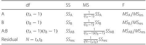
Table 3A general two-way ANOVA table consisting of a factorial treatment structure between factors A and B
df SS MS F
Thus, the overall test statistic under RFM (given by FA∗B) can be directly related to the overall test statis-tic under MRF (given by FA+B), see Section 1 of the Supplementary Material in Additional file 1 for details. This relationship is shown in Fig. 2c for tA = 4,tB =
3, N = 36 and overall F-statistic of FA∗B = 2, which implies an associated p-value of pA∗B = 0.075. Thus, regardless of the significance of any individual main effects, under RFM this response variable would be fil-tered out as being non-significant. However, as can be seen in Fig.2c, when the interaction term is sufficiently non-significant (and consequently one or more main effects are highly significant since the overall variance ratio is fixed at 2), MRF would correctly identify a sig-nificant response variable. Thus, RFM is a conservative approach that has the potential for prematurely filtering out responses.
By moving the filtering step of the RFM approach to post-model selection step (i.e. a rank model filter (RMF) approach as described in Additional file 1 of the Supplementary Material), this conservativeness can be mitigated, but ranking in the first step will, in general, result in a more conservative multiplicity cor-rection compared to the MRF approach that applies multiplicity corrections to the one-way test of the pre-dictive model associated with larger residual degrees of freedom.
Results
The methods derived above are demonstrated and compared through a comprehensive simulation study before being applied to the lipidomics dataset previously described. For this dataset, we also consider in detail the interpretation of such analyses through the presentation and visualisation of the output.
Simulation study
In order to comprehensively compare these methods, our simulation study considered three different designs (a 2×2 factorial treatment structure, a 3×2×4 factorial treat-ment structure and a 3×2×4 factorial treatment structure with an imposed randomized complete block structure). For each design, we varied the number of responses (500, 1000 and 20000), the number of replicates (3, 4 and 5) and the multiplicity control (FDR via Benjamini-Hochberg and FWER via Bonferroni). In addition, for the randomized complete block design responses were simulated with a block diagonal depen-dence structure. Each scenario was simulated 50 times in order to obtain representative estimates of the achieved error rates under the two methods of interest (RFM and MRF). Thus, in total, 1350 datasets were simulated cov-ering a range of design scenarios, each of which was analysed via the following four methods.
1. RFM, with Benjamini-Hochberg (B-H) multiplicity correction controlling the FDR at 5% and model selection via F-tests
2. MRF, with Benjamini-Hochberg multiplicity correction controlling the FDR at 5% and model selection via F-tests
3. RFM, with Bonferroni multiplicity correction controlling the FWER at 5% and model selection via F-tests
4. MRF, with Bonferroni multiplicity correction controlling the FWER at 5% and model selection via F-tests
To compare the RFM and MRF approaches, we investi-gated the observed error rates within the simulation study. Throughout, we focus our discussion to the analysis under a B-H multiplicity correction. Further discussion under a Bonferroni multiplicity correction is given in Section 3.3 of the Supplementary Material in Additional file1.
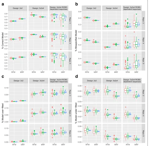
Figure 3a shows the distribution of the percentage of false positives (out of a total ofRresponses) for each sim-ulation scenario. From this, it can be seen that under the MRF, more false positives are detected than under the RFM. However, both methods appear to control the FDR (as shown empirically in Section 3.2 of the Supplementary Material in Additional file1). As the number of responses increases, the distribution of error rates tightens with little difference observed as the sample size increases. More-over, it is clear that where there is a strong dependence structure between responses there is a greater variabil-ity in the type I error rate obtained under the MRF. Since model selection is emphasised under the MRF, this approach would likely benefit by taking explicit account of the dependence structure in the modelling step, for example through a hierarchical approach. The distribu-tion of the percentage of false negatives (the number of responses falsely identified as non-significant out of a total ofRresponses) is shown in Fig.3b. Under the MRF, fewer false negatives are detected than under the RFM as pre-dicted from Fig.2c. Moreover, it can clearly be seen that as the power of the tests increases for larger sample sizes and more complex experiments, the rate of false negatives decreases.
b
a
Fig. 3Simulation Study: Overall Type I and Type II error. Under a B-H control of the FDR:aBoxplots showing the distribution of the percentage of responses (within a dataset) falsely identified as having non-constant mean response andbBoxplots showing the distribution of the percentage of responses (within a dataset) falsely identified as having a constant mean response over all treatment groups
to the rate of under-fitting for the more complex design structure (Fig.4candd). Moreover, in these more complex design scenarios, the RFM generally has a higher rate of under-fitting than the MRF (Fig.4d) providing a more par-simonious representation of the response but at the cost of a conservative filtering of overall differential expression.
Case study: Lipidomics
a
b
c
d
Fig. 4Simulation Study: Model misspecification. Under a B-H control of the FDR:aPercentage of responses with the correct model specification identified from each of the RFM and MRF approaches compared to the true generating process.bPercentage of responses with a model misspecification identified from each of the RFM and MRF approaches compared to the true generating process.cPercentage of responses that have been over-fitted (the fitted model includes all terms from the true generating process with additional terms) under the RFM and MRF approaches.dPercentage of responses that have been under-fitted (the fitted model includes only a subset of terms, and no others, from the true generating process) under the RFM and MRF. A model misspecification is defined to be a model that differs from the true generating process in a way not captured by over- or under-fitting. Red, green and blue correspond to simulations of 500, 1000 and 20000 responses respectively
showing differential expression between treatments under RFM, whilst under MRF all 131 lipids were identified. However, discrepancies between the methods become apparent when assessing the selected predictive model, with around 4% fewer lipids found to have a significant interaction term under RFM compared with MRF. These
differences were exacerbated with the application of a more stringent Bonferroni correction (not shown).
use high throughput technologies to identify a list of the most ‘interesting’ response variables to investigate further. In the simplest case, where comparisons are only made between two treatment conditions, comparisons are often visualised through volcano plots, which show the rela-tionship between statistical significance (often scaled log-arithmically) and biological relevance (often presented in terms of fold change to a baseline condition). This enables easy identification of the ‘most interesting’ responses that are both statistically significant and biologically rele-vant. However, for more complex explanatory (treatment) structures, it is far from clear how to identify ‘interesting’ responses.
Overall assessment
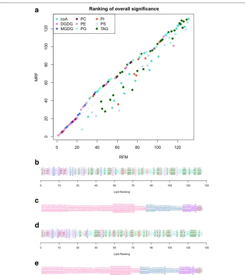
In both the RFM and MRF approaches, a one-way F-test is applied to obtain an overall level of significance. The meaning of this one-way test is fundamentally different in the two approaches since under RFM, it is a test of the saturated model, whereas under MRF, it is a test of the predictive model. Nevertheless, this measure of statistical significance can be used to rank responses. Figure5shows the discrepancy in the ranking of responses from the two methods, with RFM giving a greater rank to response variables with significant interaction components, whilst MRF gives greater rank to responses with parsimo-nious predictive models (relative to the corresponding saturated model).
In addition, these approaches can be used to charac-terise the response variables through the identified predic-tive model. For example, the lipidomics response variables can be categorised into 8 different groups, where each group contains response variables with the same tive model. As shown in the simulation study, the predic-tive models identified by the two approaches differ and so different categorisations of the response variables are obtained as shown in Fig.5cande.
More meaningful insight can be obtained by coupling these overall measures of significance with measures of biological relevance. One approach to obtaining measures of biological relevance is through predictions obtained from the predictive model selected in the two-step analy-sis procedures. Since an overall assessment of significance based on the saturated model (as under RFM) may have very little relevance to predictions from the predictive model, the overall assessment of significance based on the predictive model (as under MRF) should be used.
Model predictions are a useful way of defining biological relevance, for example through the predicted fold change between two treatment conditions. However, when there are more than two treatment conditions multiple mea-sures of biological relevance can be obtained and the most meaningful comparisons will be context specific. For example, the treatment condition of theArabidopsis
variety Columbia under no salt stress can be considered as a baseline or default status. In this scenario, a measure of biological relevance can be obtained as the predicted fold change (in each treatment condition) from the base-line level. This results in a series of pairwise comparisons to a baseline and can be represented through asetof vol-cano plots (Fig.6a) where the measure of significance is constant across all plots, but with each subplot reflect-ing the fold change from baseline due to each individual treatment condition. Consequently, the set of ‘important’ response variables can be identified as those that are sta-tistically significant overall and have a fold change greater than some threshold in at least one treatment relative to the baseline. From this, it can be seen that the conditions identifying the greatest number of ‘important’ response variables are associated with differences in lipid abun-dance between the genotype Eutrema compared to the abundance in the genotype Columbia. However, these pairwise comparisons make no use of the explanatory structure and it is arguably more appropriate either to obtain a structured summary (see below) or to obtain a single overall measure of biological relevance. For exam-ple, Fig. 6b shows two volcano plots, where biological relevance is calculated as the maximal fold increase (and decrease) in any treatment condition compared to the baseline, thus giving a single ranking of ‘importance’ over the response variables.
It is important to emphasise that the (biologically rel-evant measures of ) differences are not necessarily statis-tically significant, and that the aim here is to produce a ranking considering a measure of overall statistical significance coupled with a notion of overall biological relevance. For example, lipid X30.0 is considered to be important as it shows both differential expression (a sta-tistically significant one-way analysis) and the largest fold increase in any treatment condition compared to the base-line of no salt stress in Columbia.
Marginal assessment
With a complex treatment structure, it will usually be preferable to assess statistical significance for particular treatment terms in the linear model in order to answer specific questions associated with the design of the treat-ment structure. In a univariate framework, there are three approaches to do this;
1. Assess individual model terms through the appropriately structured ANOVA (or equivalent analysis framework),
2. Incorporate a set of orthogonal contrasts into the treatment structure of the linear model and assess these terms (e.g. through ANOVA),
a
b
c
d
e
a
b
Fig. 6Lipidomics Case Study: Overall Assessment under the MRF.aCoupling the overall measure of statistical significance (of the one-way test under MRF after a Benjamini-Hochberg multiplicity correction) with measures of biological relevance calculated as the predicted fold change in abundance compared to the baseline treatment of no salt stress for the variety Columbia (Col).bCoupling the overall measure of statistical significance (of the one-way test under MRF after a Benjamini-Hochberg multiplicity correction) with a generalised measured of biological relevance calculated as the maximal fold increase (or decrease) under any treatment condition compared to the baseline treatment of no salt stress for the variety Columbia (Col). Red lines indicate ap-value of 0.05. Green lines indicate a fold change of 4
In what follows, we consider extensions of only the first two approaches to the mass univariate framework. There are a multitude of reasons for not considering the third (see, for example, references and discussion in Chapter 8 of [27]).
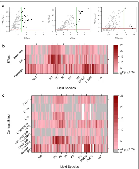
In contrast to the overall assessments of the previous section, it is now of interest to make multiple assessments for each response variable. For example, consider the subset of lipids found to have two significant main effects but no significant interaction (under RFM). The response variables can be ranked by the significance of the first factor (the variety effect) and also by the significance of the second factor (the salt effect). Unsurprisingly, these give very different rankings of the lipids, both of which are of biological interest. To give meaning to these mea-sures of statistical significance, an associated measure of biological relevance is required. For a two-level factor, this is straightforward and simply results in the standard volcano plot of difference (often presented in fold change) vs. significance. For a factor with more than two levels, a similar approach to the overall assessment could be used. For instance defining relevance as a maximal fold change to a baseline or, where no baseline exists, the max-imal fold change between pairs of treatment conditions. However, neither of these approaches maintain the factor definition of a marginal assessment. A natural alternative is to generalise the notion of biological relevance from simple comparative predictions to estimated effects. Explicitly, relevance can be defined by √MST, where
MST is the treatment mean square for the explanatory term T. A larger value of the treatment mean square indicates a greater variation in the mean response of the levels of the treatment factor. Consequently, a biologically relevant threshold,ThresB, can be defined such that only response variables showing aMST > ThresBare deemed relevant. Moreover, under the RFM, each treatment mean square is explicitly tested against the null hypothesis thatMST/MSres = 1 at a significance level corrected for
multiplicity according to the associated one-way analysis. Since the residual mean square, MSres, is an estimate
of background variation, this hypothesis test provides the corresponding assessment of statistical significance having adjusted for multiplicity. Thus, a generalisation of the volcano plot is obtained (Fig. 7a) for individual explanatory terms.
In addition, the adjusted p-values for each treatment term can be obtained for each response variable. This is shown for the lipidomic data in Fig. 7b, where lipids can be identified according to the most significant treat-ment factor. For instance, the majority of PC lipids are seen to have more significant effects associated with salt stress, while MGDG lipids have more significant effects associated with differences in genotype.
The above assessment of individual factors extends the analysis obtained from ANOVA to the mass univariate framework. In a similar way to a single univariate analysis, a greater level of detail can be obtained by decompos-ing the explanatory model structure. If each term within the linear model can be parameterised into a set of one
degree of freedom terms (or contrasts), than marginal assessment boils down to a set of hypothesis tests that can be directly related to a treatment difference and hence tra-ditional volcano plots can be used. In practice, this will rarely occur but as exemplified in the lipidomics experi-ment, contrasts can be included to extract a greater level of detail. For example, rather than simply analysing the factor associated with three levels of salt stress, this factor can be decomposed into two parts in order to test for evi-dence of a linear trend and deviations from such a trend in the quantitative levels of salt stress. Similarly, the fac-tor associated with four different genotypes ofArabidopsis
can be decomposed into two parts in order to test for a) differences in ecotypes (Eutrema vs. Others) and b) differ-ences in genotypes within the same ecotype (Columbia, Ta-0 and Shadara). These effects are shown in Fig.7cand again groups of responses showing similar patterns can be extracted.
It is clear that as more complex models are consid-ered this approach of marginal assessment becomes more involved. However, the generalised visualisations extend-ing the interpretation of ANOVA into three dimensions (term, effect size, response) can greatly aid the biological interpretation.
Discussion
In this paper, two methods have been introduced for incorporating multiplicity corrections in a mass uni-variate analysis for non-trivial explanatory (treatment) structures. Each approach has its own advantages and the choice between them will depend upon the con-text of any analysis. The RFM approach has been shown to be conservative in identifying statistically significant response variables, as multiplicity is applied to the one-way test of the saturated model, whereas the MRF approach overcomes this conservativeness through an inflation of the residual degrees of freedom due to a one-way test of the predictive model. Inflating the residual degrees of freedom under MRF may not always be desir-able and an alternative would be to partition the treatment sums of squares into two parts, one associated with the one-way treatment structure of the predictive model and the other associated with a ‘lack-of-fit’ term. In this way, a one-way test of the predictive model can be defined whilst maintaining the residual degrees of freedom for which the experiment was designed.
a
b
c
individual treatment effects or an incorporation of con-trast effects are more naturally expressed in the RFM framework.
Alternative approaches
In this paper, attention has been focussed on control-ling the multiplicity of tests of the full explanatory model over the R response variables, i.e. at the response vari-able level within an experiment, through a stage-wise hypothesis testing procedure. Alternatives to this stage-wise paradigm can be found in the literature, but have lim-itations to the response-level interpretation. Specifically, rather than controlling the FDR at the response-level, an alternative would be to correct for multiplicity over theR
responses for each of thepexplanatory terms, i.e. at the explanatory term level within an experiment.
The naïve approach might consider that forp explana-tory terms over R response variables, a total of R× p
tests are required. As such, a global multiplicity correc-tion over this full set of R× p tests could be applied. However, this approach will be vastly over-conservative. Moreover, for all but the simplest form of correction, interpretation becomes difficult as each of the explana-tory terms for a single response variable will be assessed at a different level of significance as, for example, under a Benjamini-Hochberg correction. This prevents the use of a model-based interpretation that combines statistical significance with biological relevance as in the examples above.
In orthogonal balanced designs, it is conceivable that controlling multiplicity for each explanatory term sep-arately is desirable. Specifically, p separate multiplicity corrections can be applied for each of thepexplanatory terms. This then results in the identification of groups of responses that are statistically significant for each sep-arate explanatory term as implemented in [15]. As with the approaches derived in this paper, an additional model selection step can be included to base the multiplicity corrections on the predictive rather than saturated mod-els. Applying these approaches to the simulated data in scenario 1 (Section 4 of the Supplementary Material in Additional file 1), large discrepancies can be seen, par-ticularly in the assessment of significance of the main effects. This is unsurprising, since this Model, Subset, Filter (MSF) approach does not respect the ‘bottom-up’ marginality interpretation of the ANOVA, with main effects potentially omitted without the prior removal of the associated interaction terms. Moreover, the final inter-pretation becomes limited, as again one cannot analyse the output in a model-based framework as the assessment of individual terms is not consistent within a response variable.
Both the global multiplicity corrections (for allR×p
tests) and separate multiplicity corrections (over allptests
for each ofRterms) are incorporated in the limma package [24] for differential expression analysis of RNAseq and microarray data.
Extensions
This paper has focussed attention on designed experi-ments where all terms within a linear model are factors and the associated analysis can be extracted through ANOVA. In practice, many ’omics datasets may be bet-ter suited to albet-ternative univariate analysis approaches such as linear mixed models (to account for unbalanced designs), linear and generalized linear models to account for covariates or non-normal responses and hierarchi-cal models to account for known dependence structures. Regardless of the complexity of the individual univariate technique, so long as there is a clear definition of a satu-rated and predictive model, the principles introduced in this paper will hold.
Conclusions
Mass univariate approaches provide a valuable comple-ment to multivariate techniques to analyse and inter-pret ’omics data. In particular, univariate approaches are often well developed for problematic data, for instance, in dealing with missing values, unequal replication, unbalanced designs and autocorrelated error structures, which can be difficult to incorporate in a multivari-ate setting. Moreover, mass univarimultivari-ate approaches enable statistical significance and biological relevance to be assessed at an individual response variable level in addition to the profile level assessment obtained through a multivariate analysis.
However, as demonstrated in this paper, when analysing ’omics data through a mass univariate approach, a choice of procedures for incorporating multiplicity corrections is available. To gain a deeper understanding of the mech-anisms underlying a particular response variable, it is particularly important to assess the full treatment struc-ture of the design rather than the simplified one-way analysis common in the literature. When coupled with an approach to control the multiplicity rate, different analy-sis approaches give more or less influence to either fitting the predictive model or correcting for multiplicity. Thus, it is important to be aware of the implicit choice that is being made.
procedures for obtaining the predictive model whilst also incorporating multiplicity corrections have been intro-duced and illustrated on data. The approach to use will be driven by the specific aims of the analysis, namely whether a marginal or overall assessment is most appropriate.
Since this choice in methods arises due to the pres-ence of non-trivial (more complex) explanatory treatment structures, this consideration will become increasingly important as the ability to include more complex treat-ment structures and collect observational covariates becomes more accessible due to the influx of accessible ’omics technologies.
Additional files
Additional file 1: Supplementary Material.Section 1Equating variance ratios.Section 2Description of the RMF approach.Section 3Simulation study:Section 3.1Data generation,Section 3.2False discovery rates,
Section 3.3Results under a Bonferroni correction of the FWER,Section 3.4
Comparison to limma approaches,Section 3.5Comparison of MSF approaches. (PDF 330 kb)
Additional file 2:Lipidomics model assessment. Table containing the overall assessment of statistical significance and the model fitted for each lipid under both RFM and MRF. (PDF 8 kb)
Abbreviations
ANOVA: Analysis of variance; B-H: Benjamini-Hochberg; FDR: False discovery rate; FWER: Family-wise error rate; MRF: Model, rank, filter; OFDR: Overall false discovery rate; PFER: Per-family error rate; RFM: Rank, model, filter; RCBD: randomized complete block design
Acknowledgements
The authors acknowledge Louise Michaelson, Richard Haslam and Fredrick Ibinda for their contributions to the understanding of the lipid data and the development of the statistical thinking. KLH would like to thank attendees of the 2016 CIBB conference for valuable discussions that contributed to this manuscript.
Funding
This work has been part funded from the Designing Future Wheat (BBS/E/C/000I0210) and Tailoring Plant Metabolism (BBS/E/C/000I0420) strategic programmes funded by the Biotechnology and Biological Sciences Research Council. Publication costs were funded from the Biotechnology and Biological Sciences Research Council’s Open Access Grant to Rothamsted Research.
Availability of data and materials
The datasets used during the current study are available from the corresponding author on reasonable request.
About this supplement
This article has been published as part ofBMC BioinformaticsVolume 19 Supplement 7, 2018: 12th and 13th International Meeting on Computational Intelligence Methods for Bioinformatics and Biostatistics (CIBB 2015/16). The full contents of the supplement are available online athttps://
bmcbioinformatics.biomedcentral.com/articles/supplements/volume-19-supplement-7.
Authors’ contributions
KLH ran the simulations, analysed the data, prepared the manuscript and derived the formulae. AM prepared the manuscript and derived the formulae. Both authors read and approved the final manuscript.
Ethics approval and consent to participate
Not applicable.
Competing interests
The authors declare that they have no competing interests.
Publisher’s Note
Springer Nature remains neutral with regard to jurisdictional claims in published maps and institutional affiliations.
Published: 9 July 2018
References
1. Checa A, Bedia C, Jaumot J. Lipidomic data analysis: tutorial, practical guidelines and applications. Anal Chim Acta. 2015;885:1–16. 2. Wheelock ÅM, Wheelock CE. Trials and tribulations of ’omics data
analysis: assessing quality of simca-based multivariate models using examples from pulmonary medicine. Mol BioSyst. 2013;9(11):2589–96. 3. Higashi Y, Okazaki Y, Myouga F, Shinozaki K, Saito K. Landscape of the
lipidome and transcriptome under heat stress in arabidopsis thaliana. Sci Rep. 2015;5.http://dx.doi.org/10.1038/srep10533.
4. Vu HS, Shiva S, Roth MR, Tamura P, Zheng L, Li M, Sarowar S, Honey S, McEllhiney D, Hinkes P, et al. Lipid changes after leaf wounding in arabidopsis thaliana: expanded lipidomic data form the basis for lipid co-occurrence analysis. Plant J. 2014;80(4):728–43.
5. Curtis TY, Muttucumaru N, Shewry PR, Parry MA, Powers S, Elmore JS, Mottram DS, Hook S, Halford NG. Effects of genotype and environment on free amino acid levels in wheat grain: implications for acrylamide formation during processing. J Agric Food Chem. 2009;57(3):1013–21. 6. Habash DZ, Baudo M, Hindle M, Powers S, Defoin-Platel M, Mitchell R,
Saqi M, Rawlings C, Latiri K, Araus JL, et al. Systems responses to progressive water stress in durum wheat. PloS ONE. 2014;9(9):108431. 7. Min B, Gonzalez-Thuillier I, Powers S, Wilde P, Shewry PR, Haslam RP.
Effects of cultivar and nitrogen nutrition on the lipid composition of wheat flour. J Agric Food Chem. 2017;65(26):5427–5434.https://doi.org/ 10.1021/acs.jafc.7b01437.
8. Dudoit S, Shaffer JP, Boldrick JC. Multiple hypothesis testing in microarray experiments. Stat Sci. 2003;18:71–103.
9. Dudoit S, van der Laan MJ. Multiple Testing Procedures with Applications to Genomics. New York: Springer; 2008.
10. Austin SR, Dialsingh I, Altman NS. Multiple hypothesis testing: A review. J Indian Soc Agric Stat. 2014;68(2):303–14.
11. Ge Y, Dudoit S, Speed TP. Resampling-based multiple testing for microarray data analysis. Test. 2003;12(1):1–77.
12. Cheverud JM. A simple correction for multiple comparisons in interval mapping genome scans. Heredity. 2001;87(1):52–8.
13. Li J, Ji L. Adjusting multiple testing in multilocus analyses using the eigenvalues of a correlation matrix. Heredity. 2005;95:221–7.https://doi. org/10.1038/sj.hdy.6800717.
14. Moskvina V, Schmidt KM. On multiple-testing correction in genome-wide association studies. 2008;32:567–73.https://doi.org/10.1002/gepi.20331. 15. Rudd J, Kanyuka K, Hassani-Pak K, Derbyshire M, Devonshire J, Saqi M, Desai N, Powers S, Hooper J, Ambroso L, Bharti A, Farmer A, Hammond-Kosack KE, Dietrich RA, Courbot M. Transcriptome and metabolite profiling the infection cycle of Zymoseptoria tritici on wheat (Triticum aestivum) reveals a biphasic interaction with plant immunity involving differential pathogen chromosomal contributions, and a variation on the hemibiotrophic lifestyle definition. Plant Physiol. 2015;167(3):1158–85. 16. Hammer P, Banck M, Amberg R, Wang C, Petznick G, Luo S, Khrebtukova
I, Schroth G, Beyerlein P, Beutler A. mRNA-seq with agnostic splice site discovery for nervous system transcriptomics tested in chronic pain. Genome Res. 2010;20(6):847–60.https://doi.org/10.1101/gr.101204.109. 17. Ren S, Peng Z, Mao J-H, Yu Y, Yin C, Gao X, Cui Z, Zhang J, Yi K, Xu W,
Chen C, Wang F, Guo X, Lu J, Yang J, Wei M, Tian Z, Guan Y, Tang L, Xu C, Wang L, Gao X, Tian W, Wang J, Yang H, Wang J, Sun Y. RNA-seq analysis of prostate cancer in the Chinese population identifies recurrent gene fusions, cancer-associated long noncoding RNAs and aberrant alternative splicings. Cell Res. 2012;22(5):806–21.https://doi.org/10.1038/ cr.2012.30.
distinct behavioral and neurochemical profiles in the orbitofrontal cortex of rats: Implications for neural function. Proteomics. 2016;16(22):2894–910. 19. Santos C, Maximiano MR, Ribeiro DG, Oliveira-Neto OB, Murad AM,
Franco OL, Mehta A. Differential accumulation ofXanthomonas campestrispv.campestrisproteins during the interaction with the host plant: Contributions of anin vivosystem. Proteomics. 2017.https://doi. org/10.1002/pmic.201700086.
20. Hur M, Campbell AA, Almeida-de-Macedo M, Li L, Ransom N, Jose A, Crispin M, Nikolau BJ, Wurtele ES. A global approach to analysis and interpretation of metabolic data for plant natural product discovery. Nat Prod Rep. 2013;30(4):565–83.https://doi.org/10.1039/c3np20111b. 21. Benjamini Y, Bogomolov M. J R Stat Soc Ser B (Stat Methodol). 2014;76(1):
297–318.
22. Benjamini Y, Heller R. Screening for partial conjunction hypotheses. Biometrics. 2008;64(4):1215–22.
23. Jiang H, Doerge RW. A two-step multiple comparison procedure for a large number of tests and multiple treatments. Stat Appl Genet Mol Biol. 2006;5(28).https://doi.org/10.2202/1544-6115.1223.
24. Ritchie ME, Phipson B, Wu D, Hu Y, Law CW, Shi W, Smyth GK. limma powers differential expression analyses for rna-sequencing and microarray studies. Nucleic Acids Res. 2015;43(7):47.
25. Heller R, Manduchi E, Grant GR, Ewens WJ. A flexible two-stage procedure for identifying gene sets that are differentially expressed. Bioinformatics. 2009;25(8):1019–25.
26. Van den Berge K, Soneson C, Robinson MD, Clement L. A general and powerful stage-wise testing procedure for differential expression and differential transcript usage. bioRxiv. 2017.https://doi.org/10.1101/ 109082.