www.nonlin-processes-geophys.net/19/127/2012/ doi:10.5194/npg-19-127-2012
© Author(s) 2012. CC Attribution 3.0 License.
Nonlinear Processes
in Geophysics
On closure parameter estimation in chaotic systems
J. Hakkarainen1,2,*, A. Ilin3,*, A. Solonen1,2,*, M. Laine1, H. Haario2, J. Tamminen1, E. Oja3, and H. J¨arvinen1 1Finnish Meteorological Institute, Helsinki, Finland
2Lappeenranta University of Technology, Lappeenranta, Finland 3Aalto University School of Science, Espoo, Finland
*These authors contributed equally to this work.
Correspondence to: J. Hakkarainen ([email protected])
Received: 21 November 2011 – Revised: 3 February 2012 – Accepted: 7 February 2012 – Published: 15 February 2012
Abstract. Many dynamical models, such as numerical weather prediction and climate models, contain so called clo-sure parameters. These parameters usually appear in physical parameterizations of sub-grid scale processes, and they act as “tuning handles” of the models. Currently, the values of these parameters are specified mostly manually, but the increasing complexity of the models calls for more algorithmic ways to perform the tuning. Traditionally, parameters of dynamical systems are estimated by directly comparing the model sim-ulations to observed data using, for instance, a least squares approach. However, if the models are chaotic, the classical approach can be ineffective, since small errors in the initial conditions can lead to large, unpredictable deviations from the observations. In this paper, we study numerical methods available for estimating closure parameters in chaotic mod-els. We discuss three techniques: off-line likelihood calcula-tions using filtering methods, the state augmentation method, and the approach that utilizes summary statistics from long model simulations. The properties of the methods are stud-ied using a modifstud-ied version of the Lorenz 95 system, where the effect of fast variables are described using a simple pa-rameterization.
1 Introduction
Many dynamical models in atmospheric sciences contain so called closure parameters. These parameters are usu-ally connected to processes that occur on smaller and faster scales than the model discretization allows. For instance, the computational grid used in modern climate and numerical weather prediction (NWP) models is too coarse to directly model cloud micro-physics and many cloud-related phenom-ena are therefore represented by parameterization schemes. For example, consider the cloud shortwave optical proper-ties, which are related to the cloud liquid water amount, and
affect the shortwave radiation fluxes in atmospheric models. These properties can be specified with parameters, such as the mean effective radius of cloud water droplets (Martin et al., 1994).
The closure parameters act as “tuning handles” of the models. Parameter tuning is particularly necessary whenever new and improved parameterized processes are implemented into the models. Currently, the parameters are usually pre-defined by experts using a relatively small number of model simulations. This tuning procedure is somewhat subjective and therefore open for criticism.
In this paper, we discuss different algorithmic ways to es-timate the tuning parameters, that is, how to find the opti-mal closure parameters by fitting the model to available ob-servations. While this problem has not been studied much, there are a few recent papers that address the problem in the context of climate modeling (Jackson et al., 2008; Villagran et al., 2008; J¨arvinen et al., 2010; Sexton et al., 2011). Nu-merical weather prediction (NWP) is considered to be more of an initial value problem than a parameter estimation prob-lem (Annan and Hargreaves, 2007) and tuning of closure pa-rameters is in general done manually by using samples of test forecasts. In a recently proposed approach, NWP parame-ter estimation is embedded into ensemble prediction systems (J¨arvinen et al., 2011; Laine et al., 2011).
To fix the notation, let us assume for simplicity that a dy-namical model can be described by a discrete state space model
xk=M(xk−1,θ) (1)
zk=K(xk), (2)
wherex denotes the state of the system, the model opera-torM solves the equations that describe the dynamics of the system, k is the index of the time, z are the variables that can be observed, K is the observation operator and θ
denotes the (closure) parameters. The model operatorMis assumed to contain everything that is needed to simulate the system, including also as external forcing terms and bound-ary conditions. In the real-world setting, we would like to tune parametersθ of the model in Eqs. (1)–(2) using a set of available observationsy= {y1,...,yn}taken at some time
instances{t1,...,tn}. Note thatyare measured values, while zare simulated values of the same variables.
In parameter estimation, we follow the Bayesian method-ology, in which the knowledge about the unknown parame-ters is inferred from the posterior distributionp(θ|y): p(θ|y)∝p(θ)p(y|θ), (3) which is evaluated using the priorp(θ)and the likelihood p(y|θ). The likelihood function specifies how plausible the observed data are given model parameter values. Therefore, defining a proper likelihood function is the central problem in parameter estimation. The prior contains the information that we have about the parameters based on the accumulated in-formation from the past. For an introduction to Bayesian es-timation, see, for example, the book by Gelman et al. (2003). Traditionally, parameters of dynamical systems are esti-mated by comparing model simulations to observed data us-ing a measure such as a sum of squared differences between
zandy. This corresponds to the assumption that the obser-vations are noisy realizations of the model values. The prob-lem in applying these techniques directly to chaotic systems is that the dynamically changing model statexis not known exactly, and small errors in the state estimates can grow in an unpredictable manner, making direct comparisons of model simulations and observations meaningless over long time pe-riods.
In this paper, we consider three ways to estimate the clo-sure parameters of chaotic models. In the first approach, ob-servations and model simulations are summarized in the form of statistics, which are typically some temporal and spatial averages of the data. The likelihood model is constructed in terms of the summary statistics such that model parameters producing statistics that are closer to the observed statistics would have higher likelihood. This kind of an approach is employed in climate model parameter estimation in several recent studies (Jackson et al., 2008; J¨arvinen et al., 2010; Sexton et al., 2011). In the summary statistics approach, the problem of chaotic behavior can be alleviated, since the
0 2 4 6 8 10 12 14 16 18 20
−5 0 5 10
Time
State variable
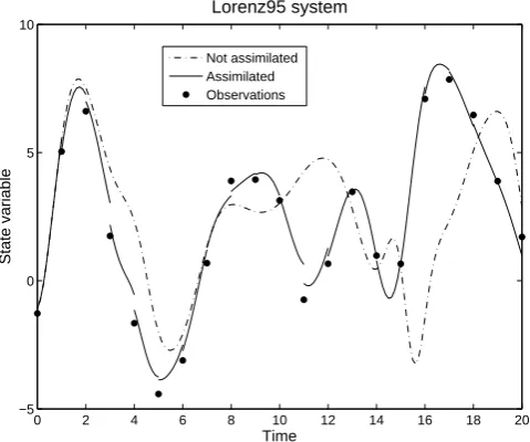
Lorenz95 system
Not assimilated Assimilated Observations
Fig. 1. An illustration of sequential data assimilation in a chaotic
system. After some time the control run, even with optimal param-eter values, gets “off track” due to chaos. Data assimilation keeps the model in the same trajectory with the data.
statistics computed from long simulations are less dependent on the initial conditions than the specific values of the state variables.
The other two approaches are based on embedding the pa-rameter estimation techniques into dynamical state estima-tion (data assimilaestima-tion) methods that constantly update the model state as new observations become available. Thus, the model is kept in the vicinity of the data, and the problems caused by chaotic behavior can be alleviated. This is illus-trated in Fig. 1 by running the Lorenz system – that is used for experimentation in Sect. 5 – two times from the same ini-tial values, with and without data assimilation. One can see that the model run without assimilation eventually deviates from the trajectory of the observations.
parameter estimation of stochastic models (see, e.g. Kivman, 2003; Singer, 2002; Dowd, 2011), but less studied in connec-tion with deterministic, chaotic systems.
The paper is organized as follows. In Sect. 2, we present the methodology for the summary statistics approach. The likelihood approach is discussed in Sect. 3, and the sequen-tial parameter estimation via state augmentation is presented in Sect. 4. In Sect. 5, the case study setup and numerical re-sults are presented. In Sect. 6 we discuss some specific issues related to the properties of the methods. Section 7 concludes the paper.
2 Likelihood based on summary statistics
Several recent studies (Jackson et al., 2008; J¨arvinen et al., 2010; Sexton et al., 2011) on parameter estimation in cli-mate models formulated the likelihood in terms of summary statistics. The advantage of this approach is that it is compu-tationally feasible and rather straightforward to implement. It avoids the problem of chaotic behavior as in sufficiently long simulations the effect of the initial values diminishes.
In this approach, the observations are transformed to a set of summary statisticss=s(y1:n), wherey1:ndenotes all
ob-servations fornsteps of the simulation model Eqs. (1)–(2). The posterior distribution of model parametersθis evaluated as
p(θ|s)∝p(θ)p(s|θ). (4) The likelihoodp(s|θ)is constructed so that modelsθ pro-ducing summary statisticssθwhich are close to the observed valuessget higher probability. Here,sθ=s(zθ,1:n)denotes
the summary statistics computed from datazθ,1:n simulated
fornsteps with model parametersθ. The approach is related to approximate Bayesian computation (ABC, see, e.g. Cor-nuet et al., 2008), where summary statistics are used to do statistical inference in situations where the exact likelihood is intractable.
2.1 Matching observed and simulated statistics
When the simulated and observed summary statistics are di-rectly matched, the likelihood can be formulated, for in-stance, as
p(s|θ)∝exp
−1
2C(s,sθ)
, (5)
whereC(s,sθ)is a cost function penalizing the misfit
be-tweens andsθ. For example, one could use the Gaussian
assumption yielding the form
C(s,sθ)=(s−sθ)T6−1(s−sθ), (6)
where the covariance matrix6 takes into account possible correlations between the summary statistics. When some of
the correlations are ignored (Eq. 6) becomes a sum of mul-tiple terms. For example, in J¨arvinen et al. (2010) the cost function was similar to
C(s,sθ)=(sg−s g θ)
2/σ2 g
+
12
X
t=1
X
i,k
sikt−siktθ T6ikt−1sikt−siktθ , (7)
wheresgis the annual global mean of the net radiative flux at the top of the atmosphere (TOA) and sikt are zonal and monthly averages of thek-th variable computed for latitude iand montht. The first term in Eq. (7) penalizes unstable models which have an unrealistic balance of the global-mean TOA radiation, whereas the second term ensures a realistic annual cycle for the radiation. The same statistics computed from simulated data are denoted bysθgandsiktθ .
The goal of the studies by J¨arvinen et al. (2010) was to ex-plore the uncertainty of the parameters which have a large ef-fect on the radiative balance and therefore only the net radia-tive flux at TOA was used to compute the zonal and monthly averages siktin Eq. (7). In Jackson et al. (2008), several vari-ables were included in the cost function and the covariance matrix6iktwas formulated in terms of a few leading empir-ical orthogonal functions (EOFs).
One problem of the direct matching of observed and sim-ulated statistics is that the resulting likelihood Eq. (5) may not be a smooth function of the parameters, as will be seen in the experimental results (e.g. Fig. 2). A possible reason for this are the random effects caused by the finite length of the simulations. The noise in the objective function may compli-cate the parameter estimation procedure. Another problem is that the matching approach is not based on a well justified statistical model for the summary statistics: it is not easy to define what values for the summary statistics are “good” in the statistical sense. For example, it is not straightforward to select the scaling parameter6iktin Eq. (7).
2.2 Fitting a probabilistic model for summary statistics
The problems mentioned above can be partly overcome by building a probabilistic model for the summary statistics. The summary statistics are treated as random variables which are systematically affected by varying the model parameters
θ:
sθ=f(θ)+, (8)
for f include polynomials, radial basis function networks and multi-layer perceptrons.
Thus, prior to constructing the likelihood, the model has to be simulated many times with different parameter values se-lected over a suitable range. This is computationally expen-sive, but a necessary step. The likelihood is then constructed as
s|θ∼N (f(θ),6). (9)
One difficulty of learning Eq. (8) is that the set of all possi-ble statistics insθis highly multidimensional while the num-ber of examples to train the emulator Eq. (8) is potentially limited because of the high computational costs of model simulations. This problem can be solved by reducing the number of summary statistics somehow before training the model Eq. (8). The simplest way is to consider only a linear combination of the summary statistics, which means neglect-ing the variability of summary statistics outside a selected subspace. Thus, Eq. (8) is replaced by
Ws=f∗(θ)+∗, (10)
where W is a properly chosen matrix and the likelihood is formulated in terms of the projected data:
Ws|θ∼N (f∗(θ),6∗). (11)
Sexton et al. (2011), computed W using principal compo-nent analysis (PCA) and the dimensionality of the summary statistics was reduced from 175 000 to only six. Thus, the cri-terion for dimensionality reduction used there was the maxi-mum amount of variance retained in the projected statistics. Another possible approach is to find projections Ws which are most informative about closure parametersθ. For exam-ple, canonical correlation analysis is mentioned as a more appropriate dimensionality method by Rougier (2008). In the experiments presented in Sect. 5.2.1, we find W by fit-ting a linear regression modelθ≈Wsθ to the training data
{zθi,θi}. The emulator (10) is then estimated for the pro-jected statistics. Note that one can analyze the elements of W computed to maximize correlations betweenθ andsθ in
order to have a clue on which summary statistics are affected by varying the closure parameters.
3 Likelihood with filtering methods
Traditionally, the likelihood for a parameter in non-chaotic dynamical models is calculated by comparing the model to data using a goodness-of-fit measure, such as the sum of squared differences between the model and the observations. In many cases, however, the model state is not known accu-rately and it has to be estimated together with the parame-ters. This is especially important with chaotic models, where small errors in the model state can grow quickly when the model is integrated in time.
State estimation in dynamical models can be carried out using filtering methods, where the distribution of the model state is evolved with the dynamical model and sequentially updated as new observations become available. When static parameters are estimated, filtering can be used to “keep the model on track” with the measurements. In this section, we present how the likelihood in chaotic models can be com-puted using filtering methods. First, we present the general filtering formulas and then consider the special case of Gaus-sian filters.
3.1 General formulas
Let us consider the following discrete state space model at time stepkwith unknown parametersθ:
xk ∼p(xk|xk−1,θ) (12)
yk ∼p(yk|xk) (13)
θ ∼p(θ). (14)
Thus, in addition to the unknown, dynamically changing model state xk, we have static parameters θ, from which we have some prior informationp(θ). As mentioned in the introduction, the goal in parameter estimation, in Bayesian terms, is to find the posterior distribution p(θ|y1:n)of the
parameters, given a fixed data sety1:n. Here, the notation y1:n= {y1,...,yn}means all observations forntime steps.
Filtering methods (particle filter, Kalman filters, etc.) es-timate the dynamically changing model state sequentially. They give the marginal distribution of the state given the measurements obtained until the current time k. Thus, for a given value forθ, filtering methods estimatep(xk|y1:k,θ).
Filters work by iterating two steps: prediction and update. In the prediction step, the current distribution of the state is evolved with the dynamical model to the next time step: p(xk|y1:k−1,θ)=
Z
p(xk|xk−1,θ)
×p(xk−1|y1:k−1,θ)dxk−1. (15) When the new observationyk is obtained, the model state
is updated using the Bayes’ rule with the predictive distribu-tionp(xk|y1:k−1,θ)as the prior:
p(xk|y1:k,θ)∝p(yk|xk,θ)p(xk|y1:k−1,θ). (16) This posterior is used inside the integral (15) to obtain the prior for the next time step.
Using the state posteriors obtained in the filtering method, it is also possible to compute the predictive distribution of the next observation. For observationyk, the predictive
dis-tribution, given all previous observations, can be written as p(yk|y1:k−1,θ)=
Z
p(yk|xk,θ)p(xk|y1:k−1,θ)dxk. (17)
Let us now proceed to the original task of estimating static parametersθfrom observationsy1:n, i.e., computing the
pos-terior distributionp(θ|y1:n). Applying the Bayes’ formula
and the chain rule for joint probability, we obtain
p(θ|y1:n)∝p(y1:n|θ)p(θ) (18)
=p(yn|y1:n−1,θ)p(yn−1|y1:n−2,θ)...
×p(y2|y1,θ)p(y1|θ)p(θ). (19)
In the filtering context, the predictive distributions p(yi|y1:i−1,θ)are calculated based on the marginal poste-rior of the model states, see Eq. (17).
Thus, the likelihood of the whole datay1:n can be
calcu-lated as the product of the predictive distributions of the in-dividual observations. That is, to check how well the model with parameter vectorθfits the observations, one can check how individual predictions made from the current posterior fit the next observations. The only difference to traditional model fitting is that the state distribution is updated after each measurement.
Note that the above analysis only tells how the parameter likelihood is related to filtering methods. We have not yet discussed how the parameter estimation can be implemented in practice. In order to obtain the parameter estimates, two steps are required: (a) a filtering method to compute the pos-terior density for a given parameter value and (b) a parameter estimation algorithm to obtain the estimates. In this paper, we use variants of the Kalman filter for task (a), but other fil-tering methods, such as particle filters (see, e.g. Cappe et al., 2007), could be applied as well. For task (b) there are several optimization and Monte Carlo approaches available, and the method of choice depends on the case. In our examples, we use three different methods to estimate the posterior distribu-tion: a maximum a posteriori (MAP) optimization approach with a Gaussian approximation of the posterior, a Markov chain Monte Carlo (MCMC) algorithm, and an importance sampling approach. For the sake of completeness, these al-gorithms are briefly reviewed in Appendix A.
Next, we will present how the parameter estimation is per-formed in the more familiar case, where the distributions are assumed to be Gaussian, and the extended Kalman filter (EKF) is used as the filtering method.
3.2 EKF likelihood
The extended Kalman filter is one of the most popular meth-ods for state estimation in nonlinear dynamical models. EKF is an extension to the Kalman filter (KF, Kalman, 1960), where the model is assumed to be linear.
Let us now write the state space model as follows:
xk=M(xk−1,θ)+Ek (20)
yk=K(xk)+ek. (21)
Unlike in the standard EKF, the modelM now depends on parameters θ. The model and observation errors are
assumed to be zero mean Gaussians: Ek∼N (0,CEk) and ek∼N (0,Cek).
In KF, the prediction and update steps can be written down analytically, since everything is linear and Gaussian. EKF uses the KF formulas, but the model matrix in KF is replaced by a linearization of the nonlinear model. In EKF, the pre-dictive distribution for the state at timekis
xk|y1:k−1,θ∼N (xpk,Cpk), (22)
where xpk =M(xestk−1,θ)is the posterior mean xestk−1 from the previous time evolved with the model. The prior co-variance Cpk =MθkCestk−1MθkT +CEk is the covariance of the state estimate evolved with the linearized model Mθk =
∂M(xestk−1,θ)/∂xestk−1.
In the update step, the prior in Eq. (22) is updated with the new observationyk. In the EKF formulation, the posterior is xk|y1:k,θ∼N (xestk ,C
est
k ), (23)
wherexestk and Cestk are given by the Kalman filter formulas:
xestk =xpk+Gk(yk−K(xpk)) (24)
Cestk =Cpk−GkKkCpk. (25)
Here Gk=CpkKTk(KkCpkKTk +Cek)−1 is the Kalman gain
matrix and Kk=∂K(xpk)/∂x p
k is the linearized observation
operator. The predictive distribution of measurement yk, needed in the likelihood evaluation, is given by
yk|y1:k−1,θ∼N (K(xpk),Cyk), (26) where Cyk=KCpkKT+Cek. Now, applying the general for-mula (19), the total likelihood of observingy1:n, given
pa-rametersθ, can be written as p (y1:n|θ)=p(y1|θ)
n Y
k=2
p(yk|y1:k−1,θ)
=
n Y
k=1 exp
−1
2r
T k(C
y k)
−1r k
(2π )−d/2|Cyk|−1/2
∝exp
−1
2
n X
k=1
h
rTk(Cyk)−1rk+log|Cyk| i
, (27)
whererk=yk−K(xpk)and|·|denotes the determinant. Note
that the normalization constants of the likelihood terms de-pend on θ implicitly through the covariances Cpk, and the term log|Cyk| =log|KkCpkKTk +Cek|therefore needs to be
in-cluded.
The above likelihood resembles the traditional “least squares” type of Gaussian likelihoods. The difference is that the model state is allowed to change between time steps, and the residuals are weighted by the model prediction uncer-tainty term KiCpiKTi in addition to the measurement error
likelihood often used in parameter estimation. Adding the prediction error covariances to the sum of squares terms es-sentially gives more weight to situations that are predictable, and down-weights the terms where the model prediction is uncertain, due to, e.g. chaotic behavior of the system.
If, in addition to the actual model parametersθ, the model error covariance CEis unknown, we can parameterize it and estimate its parameters from the measurements together with the model parameters. As discussed later in more detail, the ability to estimate the variance parameters is one of the ad-vantages of the likelihood approach, compared to the state augmentation and summary statistics methods.
Unfortunately, as the dimension of the model increases, EKF soon becomes practically infeasible. An approximation to EKF that can be implemented in large-scale systems is the ensemble Kalman filter (EnKF). In EnKF and its numerous variants (see, e.g. Evensen, 2007; Ott et al., 2004; Whitaker and Hamill, 2002; Zupanski, 2005), the computational issues in EKF are circumvented by using sample statistics in EKF formulas, computed from a relatively small number of en-sembles. Hence, when EnKF is used, the likelihood (27) can be computed simply by definingxpi and Cpi as sample mean and covariance matrix estimated from the ensemble.
Most implementations of the EnKF involve random pertur-bations of the model states and observations. This introduces randomness in the likelihood function (27): two evaluations with the same parameter value give different likelihood val-ues. As noted by Dowd (2011), this complicates the param-eter inference, and one has to resort to stochastic optimiza-tion methods that can handle noise in the target funcoptimiza-tion (see Shapiro et al., 2009, for an introduction). Note that some recent variants of EnKF, such as many of the so called en-semble square root filters (Tippett et al., 2003) do not involve random components, and they might be more suitable for pa-rameter estimation purposes. We test a variant called Local Ensemble Transform Kalman Filter (LETKF, Hunt et al., 2007) in the experiments of Sect. 5.
4 Parameter estimation with state augmentation
In the previous section, the parameter estimation was carried out off-line by repeatedly sweeping through the data using a filter. In state augmentation (SA), the parameters are added to the state vector and estimated on-line in the filter. In prac-tice this means that model parameters are updated together with the state, whenever new observations become available. Next, we will present how SA can be implemented with EKF. Let us consider the following state space model, where the parameter vector is modeled as an additional dynamical vari-able:
xk+1=M(xk,θk)+Ex (28)
θk+1=θk+Eθ (29)
yk+1=K(xk+1)+e. (30)
For notational convenience, we have dropped the time in-dexkfrom the error terms.
In SA, we treat the combined vectorsk= [xk,θk]T as the
state vector that is updated at each time stepk. The model for the combined vector can be written as
sk+1= ˜M(sk)+Ex,θ, (31)
whereM(˜ sk)= [M(xk,θk),θk]T andEx,θ is the error of
the augmented model M, here assumed to be zero mean˜ Gaussian with covariance matrix Cx,θ.
In EKF, we now need to linearizeM(˜ sk)with respect to sk, which results in the following Jacobian matrix:
Mk=
∂M(˜ sk) ∂sk
=
∂M(sk)/∂xk ∂M(sk)/∂θk
∂θk/∂xk ∂θk/∂θk
(32)
=
∂M(sk)/∂xk ∂M(sk)/∂θk
0 I
. (33) Now, this matrix Mk can be used in the EKF formulas.
Note that the top left term in the matrix is the linearization with respect to the actual states, which is needed in the stan-dard states-only EKF as well. In addition, the derivative with respect to the parameters is needed (the top right term).
In EKF, we also need to define the model error covariance matrix Cx,θ. In SA, this must be defined in the joint space of
the state and the parameters. The errors in the state and pa-rameters are hardly uncorrelated, but for simplicity we model them here as independent random variables, which yields a block diagonal error covariance matrix
Cx,θ=
Cx 0 0 Cθ
. (34)
The model error in the state, Cx, has a clear
interpreta-tion: it represents the statistical properties of the error that the model makes in a filter time step. However, the parameter error covariance matrix Cθ lacks such an interpretation. We
consider Cθ as an additional tuning parameter of the SA
ap-proach. Roughly speaking, increasing Cθ allows more
sud-den changes fromθk toθk+1. Note that, unlike in the full likelihood approach, the model error covariance Cx cannot
be estimated from data using SA. A simple example illus-trating this problem is shown by DelSole and Yang (2010). The effect of (and the sensitivity to) Cx,θ is studied in more
detail in the experimental section. In Appendix B, we give some theoretical discussion of the effect of the selected Cx,θ.
Conceptually, SA is straightforward, although, like noted by J¨arvinen et al. (2010), it implicitly assumes the static pa-rameters as dynamical quantities and the parameter estimates therefore change at every update step of the filter. In some ap-plications, such as numerical weather prediction (NWP), this may be critical. Operational NWP systems perform under strict requirements of timely product delivery to end-users. The “drifting” model parameters have to be therefore care-fully considered from the system reliability point-of-view.
5 Case study: parametrized Lorenz 95
In this section, we will demonstrate the discussed parameter estimation approaches using a modified Lorenz system. We start by describing the model and the experiments, and then present the results for the three different methods.
5.1 Description of the experiment
To demonstrate and compare the parameter estimation ap-proaches, we use a modified version of the Lorenz 95 ODE system, detailed by Wilks (2005). The chaotic Lorenz model (Lorenz, 1995) is commonly used as a low order test model to study estimation algorithms. The system used here is similar to the original system, but the state variablesxi are affected
by forcing due to fast variablesyj, too. The full system is
written as dxk
dt = −xk−1(xk−2−xk+1)−xk+F
− hc
b
J k X
j=J (k−1)+1
yj (35)
dyj
dt = −cbyj+1 yj+2−yj−1
−
cyj+
c bFy
+ hc
b x1+bj−1
J c
(36) wherek=1,...,K andj=1,...,J K. That is, each of the “slow” state variablesxiare forced by a sum of the additional
fast variablesyj. The fast variables have dynamics similar to
the slow variables, but they are also coupled with the slow variables. We use valuesK=40,J=8,F=Fy=10,h=1
andc=b=10, adopted from (Leutbecher, 2010).
The system (35)–(36) is considered as the “truth” and used for generating synthetic data. As a forecast model, we use a version where the net effect of the fast variables is described using a deterministic parameterization. The forecast model reads as
dxk
dt = −xk−1(xk−2−xk+1)−xk+F−g(xk,θ), (37) whereg(xk,θ)is the parameterization in which the missing
fast variablesyj are modeled using the “resolved” variables.
Here, we use a polynomial parameterization,
g(xk,θ)= d X
i=0
θixk(i), (38)
withd=1. The goal is to “tune” the parametersθso that the model fits the observations as well as possible. The param-eter estimation resembles the closure paramparam-eter estimation problem in atmospheric models: the forecast model is solved with a time step1t=0.025, which is too crude for modeling the fast variables that operate on a finer time scale.
The observations for parameter estimation are generated as follows. The model is solved with dense time stepping (1t=0.0025) for altogether 2500 days (in the Lorenz model, one day corresponds to 0.2 time units). Then Gaussian noise is added to the model output with zero mean and covari-ance(0.1σclim)2I, whereσclim=3.5 (standard deviation from long simulations). When the parameters are estimated us-ing the filterus-ing approaches, only 24 out of the 40 slow vari-ables are assumed to be observed each day. The observa-tion operator, used also in previous data assimilaobserva-tion stud-ies (Auvinen et al., 2009, 2010), picks the last three state variables from every set of five states and we thus observe states 3,4,5,8,9,10,...,38,39,40. Partial observations were assumed to emulate a realistic data assimilation setting. In the experiments with the summary statistics approach, all the 40 states are assumed to be observed because hiding some of the states would introduce problems in the computation of the statistics.
Note that with this set-up, it is possible to use the values of the fast variablesyjsimulated in the full system (35)–(36)
to estimate parametersθof the forcing model
g(xk,θ)≈
hc b
J k X
j=J (k−1)+1 yj.
We will use the term “reference parameter values” for θ
which minimize the errors of this forcing model in the least squares sense. Naturally, such fitting cannot be performed in real applications since the actual sub-grid scale forcing is not known.
5.2 Results
In this section, we will present the results using the summary statistics, likelihood and state augmentation approaches. Our emphasis is on comparing the accuracy and the properties of these different approaches.
5.2.1 Summary statistics
Matching observed and simulated statistics
As mentioned in Sect. 2.1, the simulated statistics may not be a smooth function of the parameters. One method that is rather insensitive to that kind of behavior in the likelihood is importance sampling (see Appendix A3 for details). We perform importance sampling for the two parameters[θ0,θ1] of the model Eqs. (37)–(38). First, we draw 1000 candidate values uniformly and independently for the two parameters from the intervalsθ0∈ [1.4,2.2]andθ1∈ [0,0.12]. Then, the system defined by Eqs. (37)–(38) is simulated for each can-didate value, the summary statistics are computed and the likelihood is calculated. The parameter ranges were chosen so that the shape of the posterior distribution is clearly visi-ble.
In the first experiment, the cost function was constructed around a set of summary statistics which were selected ar-bitrarily. We used six statistics: mean, variance, auto-covariance with time lag 1, auto-covariance of a node with its neighbor and cross-covariance of a node with its two neigh-bors for time lag 1. Since the model is symmetric with re-spect to the nodes, we averaged these statistics across differ-ent nodes. The cost function was
C(ˆs,sθ)= 6
X
i=1
(sˆi−sθi)2/σˆi2, (39)
wheresθi is one of the six statistics computed from data simu-lated with parametersθ, andsˆi,σˆi2are the mean and variance of the same statistics computed from a relatively long simula-tion of the full-system (35)–(36) similarly to (J¨arvinen et al., 2010) . All the 40 variablesxkwere assumed to be observed
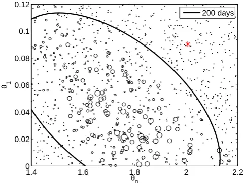
and the observation period was taken to be 200 days. Figure 2 shows the importance sampling weights obtained for the 1000 candidate values. The results show that the cost function (39) does not restrict the model parameters much and the posterior distribution is rather broad. The parameter estimates are also clearly biased: the values obtained using the knowledge of the simulated fast variables are outside the obtained distribution. Note also the “spiky” behavior of the cost function: the weights do not vary smoothly as a function of the parameters.
Likelihood based on an emulator
In the next experiment, the likelihood was computed using an emulator trained on the same set of six summary statis-tics. We again performed importance sampling of parameters θ0andθ1of the model (37)–(38) using the same 1000 can-didate values drawn fromθ0∈ [1.4,2.2] andθ1∈ [0,0.12]. The likelihood Eq. (11) was constructed using an emulator, as explained in Sect. 2.2.
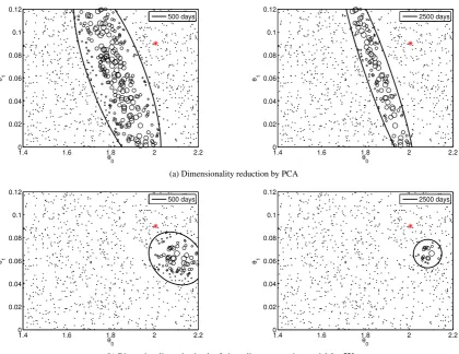
Figure 3a presents the results for the likelihood Eq. (11) in which the dimensionality reduction was performed using PCA with only two principal components retained. Figure 3b
1.4 1.6 1.8 2 2.2
0 0.02 0.04 0.06 0.08 0.1 0.12
θ0
θ 1
200 days
Fig. 2. The scatter plots of the parameter value candidates and their
likelihood (represented by the size of the markers) obtained with cost function (39). The marker size reflects the value of the weights for importance sampling. The black ellipse represents the first two moments estimated with importance sampling. The red star repre-sents the parameter values estimated by fitting the forcing model to the simulated fast variables (see Sect. 5 for details).
presents similar results for the case when the dimensionality of the features was reduced from six to two by fitting a lin-ear regression modelθ≈Wsθ and by using a feed-forward
neural network (see, e.g. Bishop, 2006) to build an emulator. There are a few remarks that we can make based on the obtained results. Using the emulator results in a posterior density which is a smooth function of the parameters, thus the problem of the spiky behavior is solved. The parame-ters found with this approach are close to the reference val-ues but there is a bias which is affected by the choice of the summary statistics. This effect is related to the known result from the field of Approximate Bayesian Computation that only using sufficient summary statistics yields the same pos-terior distribution as when the full data set is used (Marjoram and Tavar´e, 2006). A longer observational period results in a more narrow posterior distribution but the bias problem re-mains.
The results are generally sensitive to the dimensionality re-duction approach and to the number of components retained in the model. In this simple example, using more or less components leads to qualitatively similar results (biased esti-mates). In more complex cases, a cross-validation procedure (e.g. similar to Sexton et al., 2011) might be needed to esti-mate the right number of the required components.
J. Hakkarainen et al.: On closure parameter estimation in chaotic systems 135
1.4 1.6 1.8 2 2.2
0 0.02 0.04 0.06 0.08 0.1 0.12
θ 0
θ1
500 days
1.4 1.6 1.8 2 2.2
0 0.02 0.04 0.06 0.08 0.1 0.12
θ 0
θ1
2500 days
(a) Dimensionality reduction by PCA
1.4 1.6 1.8 2 2.2
0 0.02 0.04 0.06 0.08 0.1 0.12
θ 0
θ1
500 days
1.4 1.6 1.8 2 2.2
0 0.02 0.04 0.06 0.08 0.1 0.12
θ 0
θ1
2500 days
(b) Dimensionality reduction by fitting a linear regression modelθ≈Wsθ
Fig. 3.The scatter plots of the parameter value candidates and their likelihood (represented by the size of the markers) obtained with cost
function (11). The simulation length is 500 days (left) and 2500 days (right). The marker size reflects the value of the weights for importance sampling. The black ellipses represent the first two moments estimated with importance sampling. The red start represents the parameter values estimated by fitting the forcing model to the simulated fast variables (see Section 5 for details).
only two principal components are retained in the analysis and those principal components can be simulated well by the surrogate model.
700
The summary statistics approach has a few other potential problems. The choice of the summary statistics has a critical impact on the estimated parameter values. Some arbitrarily selected statistics may not be affected by varying the model parameters and the idea behind the most informative projec-705
tions is to diminish this problem. In the tuning of climate models, summary statistics often include only monthly and regional averages of some state variables, which means the focus is on how well climate models reproduce the seasonal cycle. It may be that some model parameters have little ef-710
fect on the seasonal cycle but they can be important for the overall quality of a climate model.
Thus, the summary statistics approach has a few practical problems and can result in biased estimates. We think that the essential problem is the averaging procedure in which a lot 715
of important information is lost. We argue that the sequential methods provide a more appropriate way to determine the likelihood for the parameters.
5.2.2 Likelihood calculations using filtering methods
In this section, we estimate the parameters of the forecast 720
model (37) for the Lorenz 95 system using the filtering methodology presented in Section 3.
Filtering with EKF.Implementation of EKF requires lin-earization of the model (37), which is rather straightforward in this synthetic example. As mentioned in Section 3.2, the 725
Fig. 3. The scatter plots of the parameter value candidates and their likelihood (represented by the size of the markers) obtained with cost
function (11). The simulation length is 500 days (left) and 2500 days (right). The marker size reflects the value of the weights for importance sampling. The black ellipses represent the first two moments estimated with importance sampling. The red start represents the parameter values estimated by fitting the forcing model to the simulated fast variables (see Sect. 5 for details).
only two principal components are retained in the analysis and those principal components can be simulated well by the surrogate model.
The summary statistics approach has a few other potential problems. The choice of the summary statistics has a critical impact on the estimated parameter values. Some arbitrarily selected statistics may not be affected by varying the model parameters and the idea behind the most informative projec-tions is to diminish this problem. In the tuning of climate models, summary statistics often include only monthly and regional averages of some state variables, which means the focus is on how well climate models reproduce the seasonal cycle. It may be that some model parameters have little ef-fect on the seasonal cycle but they can be important for the overall quality of a climate model.
Thus, the summary statistics approach has a few practical problems and can result in biased estimates. We think that the essential problem is the averaging procedure in which a lot of important information is lost. We argue that the sequential methods provide a more appropriate way to determine the likelihood for the parameters.
5.2.2 Likelihood calculations using filtering methods
In this section, we estimate the parameters of the forecast model (37) for the Lorenz 95 system using the filtering methodology presented in Sect. 3.
Filtering with EKF
Implementation of EKF requires linearization of the model (37), which is rather straightforward in this synthetic example. As mentioned in Sect. 3.2, the EKF filtering pro-cedure also requires the model error covariance matrix CE. We use a simple parameterization:
CE=σ2I, (40)
1.8 1.9 2 2.1 0.06
0.08 0.1 0.12
θ 1
θ0
1.8 1.9 2 2.1 −9
−8 −7 −6 −5 −4
log(
σ
2 )
0.06 0.08 0.1 0.12 −9
−8 −7 −6 −5 −4
θ1
Fig. 4. Scattering plot of parameter pairs from MCMC runs
us-ing 10 (blue), 20 (red), 50 (black) and 500 (green) day simula-tions. Clear tightening of posterior can be observed as the simu-lation length increases. The third parameter is related to the model error covariance.
In Fig. 4, the pairwise marginal distributions for the pa-rameters are illustrated using 10, 20, 50 and 500 day simu-lations. As expected, the distribution becomes tighter as the simulation length increases. Note that the posterior distri-bution is much tighter compared to the summary statistics approach (see, e.g. Fig. 3) even though almost half of the states are not observed and the filtering procedure is applied to a relatively short observation sequence. The parameter estimates are closer to the reference values obtained using the knowledge of the simulated fast variables, compared to the estimates obtained via the summary statistics approach. We also observe that the parameter distribution is approxi-mately Gaussian when sufficiently long simulations are used, as shown in Fig. 5.
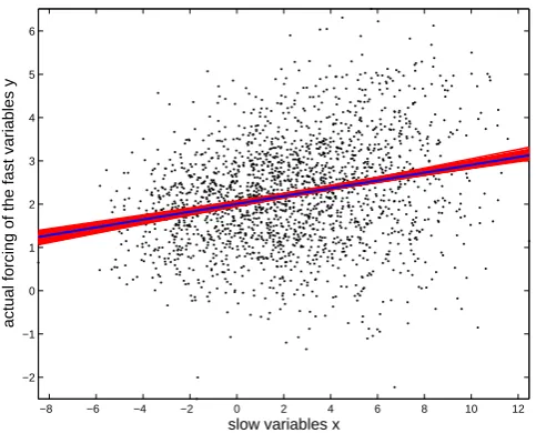
In Fig. 6, we plot the true forcing in the simulated full system (35)–(36) against the slow variables. The red lines in the figure represent the parameter values from the 50 day MCMC simulation. The blue line represent the parameter values obtained by fitting a line to the true forcing in the least squares sense. We observe good agreement with our results and the fitted line.
The estimates obtained by the likelihood approach are close to the reference values obtained using the knowledge of the fast variables. However, there is no reason to think that the reference values are optimal, for instance in the sense of forecast accuracy. Therefore, to further demonstrate that likelihood approach produces good parameter estimates, we study the effect of the parameters on the forecast skill of the model. We grid the 2-dimensional parameter space and cal-culate the average 6 day forecast skill for different parameter values. The average forecast skill is computed by making a
0.06 0.08 0.1 0.12
θ1
θ0
1.8 1.9 2 2.1
−6 −5.5 −5 −4.5 −4 −3.5
log(
σ
2)
0.06 0.08 0.1 0.12 θ1
Fig. 5. Posterior distribution using 20 day simulations with MCMC
(red dots) and Gaussian approximation (black ellipse).
−8 −6 −4 −2 0 2 4 6 8 10 12
−2 −1 0 1 2 3 4 5 6
slow variables x
actual forcing of the fast variables y
Fig. 6. Actual forcing of fast variables (black cloud). Red lines
indicate forcing from MCMC runs. Red lines in the figure represent results from the 50 day MCMC simulations. Blue line is gotten by formally fitting the parameter values in the cloud.
6 day forecast starting every 24 h for 100 days. The averaged forecast skill can be written as
f (θ)= 1
N Kσclim2
N X
i=1
kM6(xtruei ,θ)−xtruei+6k22,
where N =100, K=40 and σclim=3.5. The notation M6(xtruei ,θ) means a 6 day prediction launched from the
1.6 1.7 1.8 1.9 2 2.1 2.2 2.3 0.05
0.06 0.07 0.08 0.09 0.1 0.11 0.12 0.13 0.14
θ0
θ1
Average forecast skill
Fig. 7. An illustration of the average forecast skill. Black, red and
green dots indicate the results from 10, 50 and 500 day MCMC simulations, respectively. Blue contour colors indicate high forecast skill.
Sensitivity to model error covariance
The possibility to estimate the model error covariance CE from data is an advantage of the parameter estimation based on filtering. In data assimilation, CEis often considered as a tuning parameter which has to be selected somehow. In large scale models like NWP, the model error covariance is usually estimated in a separate procedure, and finding an effective parametrization of CEis an open question (see, e.g. Bonavita et al., 2008).
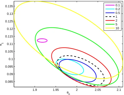
Therefore, in the following experiment, we test how spec-ifying non-optimal values for the model error covariance af-fects the quality of parameter estimation. We use the same parameterization (40) and vary the variance parameterσ2so that it is two, five and 10 times smaller or greater than the optimal value obtained in the EKF exercise with the 500 day-long simulations (see Fig. 4). We run the likelihood approach with only 50 days of data. Since the posterior distribution is approximately Gaussian, we do not perform the computa-tionally heavy MCMC runs, but compute the MAP estimate using an optimizer and calculate the Gaussian approximation of the posterior at the MAP estimate (see Appendix A).
The results are shown in Fig. 8. We observe that speci-fying the model error covariance wrongly can lead to biased parameter estimates: too small values ofσ2lead to an un-derestimated posterior covariance of the parameters and vice versa. In this specific example, we change the correct CE only by one order of magnitude and still obtain reasonable parameter estimates. For larger errors in CE, parameter esti-mates can be severely biased.
1.9 1.95 2 2.05 2.1
0.085 0.09 0.095 0.1 0.105 0.11 0.115 0.12 0.125 0.13 0.135
θ0
θ1
0.1 0.2 0.5 1 2 5 10
Fig. 8. Gaussian posterior approximations with 10, 5 and 2 times
too small and too largeσ2.
Filtering with EnKF
As discussed in Sect. 3.2, replacing the deterministic EKF with a stochastic filter, such as the EnKF, leads to a noisy likelihood function. We performed importance sampling for the two parameters similarly as in the summary statistics ex-periment in Section 5.2.1. The EnKF likelihood was evalu-ated by fixing the model error varianceσ2to the optimum found in the EKF exercise, and setting the number of ensem-ble members to 100.
In our experiment, the noise in the likelihood function dominated the statistical analysis: most of the importance weights were assigned to only a few candidate values. That is, statistical inference could not be performed properly, and the noise in the likelihood seems to be a real issue in the likelihood approach computed with EnKF. Here, we settle for plotting the negative log-likelihood surface, as was done with EnKF parameter estimation by Dowd (2011). From Fig. 9 we observe that the general pattern is good: low val-ues are found from the correct region, and a reasonable MAP estimate might be found using stochastic optimization tech-niques. However, statistical inference is complicated by the noisy likelihood. Smoothing methods could be used to al-leviate the noise in the likelihood, but this question is not pursued further here.
1.85 1.9 1.95 2 2.05 2.1 2.15 2.2 0.05
0.06 0.07 0.08 0.09 0.1 0.11
EnKF −2 × log−likelihood function values in the box with optimal σ2 (50 days)
θ0
θ1
−680 −660 −640 −620 −600 −580 −560
Fig. 9. The use of stochastic filtering method yields a noisy
hood function. The results of 50 day run using EnKF based likeli-hood function is illustrated in the Figure. The values indicate nega-tive log-likelihood times two values. White star and black ellipse is acquired from correspondent EKF likelihood calculations.
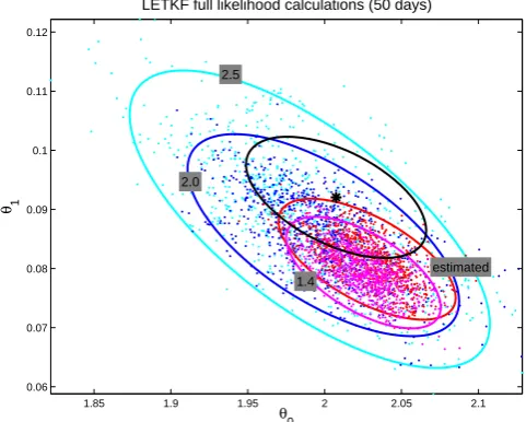
using different values for the covariance inflation parameter and a run where the inflation parameter is estimated together with the model parameters. Although there is a small bias, depending on the value of the covariance inflation parameter, the agreement with EKF calculations is rather good. Thus, deterministic ensemble filters seem to be more suitable for parameter estimation purposes.
5.2.3 State augmentation
As discussed in Sect. 4, in SA the model parameters are mod-eled as dynamical quantities, and the estimates do not con-verge to any fixed value as more observations are added. The rate at which parameter values can change from one filter time step to another is controlled by the extra tuning parame-ter, the model error covariance for the parameters, Cθ. Here,
we study how the SA method performs in parameter estima-tion and specifically how the tuning of Cθaffects the results. Tuning of the parameter error covariance
In our experiments, we use a diagonal matrix as Cθand keep
it fixed during the runs. The model error for the state vector was fixed to its “optimal value”, obtained from the likelihood experiments. In Fig. 11 we show four different runs using the EKF version of the SA method. The runs are made so that the diagonal elements of Cθ are taken to be 0.1 %, 1 %,10 %
and 100 % of the optimal parameter values acquired from the likelihood experiment. In all cases, the SA method con-verged quickly to values near the optimum. The effect of the size of Cθ was as expected. When Cθ is set to be small,
1.85 1.9 1.95 2 2.05 2.1
0.06 0.07 0.08 0.09 0.1 0.11 0.12
θ0
θ1
2.5
2.0
estimated 1.4
LETKF full likelihood calculations (50 days)
Fig. 10. Full likelihood calculations using LETKF data assimilation
method. Different MCMC runs with different covariance inflation factor together with 95 % trust ellipses. Red color indicates a run, where the factor is also estimated (mean value is 1.52). Magenta, blue and cyan colors indicate a run where covariance inflation factor is fixed to 1.4, 2.0 and 2.5, respectively. Black star and ellipse is acquired from correspondent EKF likelihood calculations.
the method reacts slowly on new data and the parameter val-ues take small steps. On the other hand, if Cθ is set large,
the method allows larger deviations, but can yield unrealistic values for the parameters. Some theoretical discussion about the effect of Cθ is given in Appendix B.
In this example, we do not observe any systematic tempo-ral variations in the parameter value. However, it is worth pointing out that the SA method could be useful in checking if such variations exist. Since the parameter trajectories are stationary, one could use the mean value of the trajectories as the final parameter estimate. In the current example, the mean is a good estimate, and it is also rather insensitive to the tuning of Cθ. In general, however, the parameter
trajec-tories cannot be interpreted in the statistical sense, since the parameter values and their variation depend entirely on the tuning of Cθ. Thus, the SA method cannot be used for
sta-tistical inference of the parameters in the same sense as the likelihood approach.
Sensitivity to model error covariance
If, on the other hand, we keep the “parameter model error covariance” Cθ fixed and vary the model error covariance Cx, the effects are somewhat different than in the likelihood
0 10 20 30 40 50 60 70 80 90 100 1
1.5 2 2.5 3 3.5
State augmentation runs
θ0
0 10 20 30 40 50 60 70 80 90 100
−0.2 −0.1 0 0.1 0.2 0.3
θ1
Fig. 11. Runs using the EKF version of the SA method, when the
di-agonal elements of Cθare taken to be 0.1 % (black), 1 % (red),10 %
(blue) and 100 % (green) of the optimal initial values. The effect of the size of Cθ was as expected. When Cθ is set to be small,
the method reacts slowly on new data and the parameter values take small steps.
the parameters: the higherσ2is, the smaller are the param-eter changes. The latter effect can be theoretically justified (see Appendix B for details).
State augmentation with EnKF
The use of ensemble based filtering methods is possible in state augmentation system. In our tests, with a large enough ensemble size, the results were similar to the EKF results. In the Lorenz system the minimum required ensemble size is roughly 50. Smaller ensemble size leads to underestima-tion of the covariances and can cause the filter to diverge. We note that state augmentation does not have the problem with the stochasticity of EnKF, which was encountered in the likelihood approach.
6 Remarks and discussion
6.1 Applicability to large scale systems
The discussed parameter estimation methods differ in their applicability to large scale systems like NWP and climate models. The summary statistics based approaches are com-putationally expensive although straightforward to imple-ment: one only needs to simulate the model, and compare the selected summary statistics of the simulations and the observations. The difficulty lies in selecting the appropri-ate summary statistics that enable the identification of the parameters.
0 50 100 150 200 250
1.7 1.8 1.9 2 2.1 2.2 2.3
State augmentation runs varying σ2
θ0
0 50 100 150 200 250
0.05 0.1 0.15
θ1
1 100 1000
1 100 1000
Fig. 12. Examples of too large model error: the model error
vari-ance is multiplied with 100 and 1000. Too large model error in state augmentation will cause bias in the parameter values. Note that the rate of change of the parameters becomes smaller as the variance grows, although Cθis kept fixed in all runs. The straight lines
rep-resent the means of the parameter trajectories.
The state augmentation and the likelihood approaches de-pend on a data assimilation system, which is often available for NWP systems, but not commonly for climate models. The state augmentation method requires modifications to the assimilation method. In deterministic assimilation systems, such as the variational approximations to EKF that are of-ten used in operational NWP systems (Rabier et al., 2000; Gauthier et al., 2007), one needs to add derivative compu-tations with respect to the parameters. If an ensemble data assimilation method is used, such as a variant of the EnKF (see Houtekamer et al., 2005) parameter perturbations need to be added. Computationally, state augmentation is econom-ical, since it requires only one assimilation sweep over the selected data.
−100 0 10 20 1000
2000 3000 4000
Full system
−100 0 10 20
1000 2000 3000 4000
Maximum likelihood estimate:
θ=[2.02 0.09]
−100 0 10 20
1000 2000 3000 4000
slow variables x
θ=[1.7 0.15]
−100 0 10 20
1000 2000 3000 4000
slow variables x
θ=[1.5 0.3]
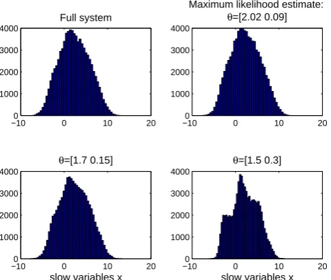
Fig. 13. Distribution of the state variables in the full Lorenz system
(top left) and in the parameterized system with maximum likelihood estimate (top left) and two arbitrarily chosen “poor” parameter val-ues (bottom row).
6.2 Climatologies with tuned parameters
In our likelihood experiment, the optimal parameter values led to improved short-range average forecast skills, as ex-pected. Another question is related to the effect of parameter tuning on the quality of long model simulations (or “clima-tologies”): the tuned parameters should, in addition to im-proving short-range forecasts, improve climatologies, too. In Fig. 13, we compare the histograms of the state variables in the full Lorenz system and in the forecast model with differ-ent parameter values. We compare the statistics of the full system to the statistics produced by the forecast model with maximum likelihood parameter estimate and two arbitrarily chosen “poor” parameter values. We observe that, in this case, the parameters tuned with the likelihood approach pro-duce also the correct climatologies. We also note that the overall statistics of the system can be quite good even with rather poor parameter values. This highlights the difficulties in choosing the correct likelihood for the summary statistics approach.
7 Conclusions
In this paper, we review three methods for parameter estima-tion in chaotic systems. In the summary statistics approach, the selected statistics computed from model simulations are compared to the same statistics calculated from observations. In the state augmentation method, unknown parameters are added to the state vector and estimated “on-line” together with the model state in a data assimilation system. In the likelihood approach, the likelihood for a parameter value is
computed by running a data assimilation method “off-line” over a selected data set. All methods were studied using a modified version of the Lorenz 95 model.
Our results indicate that the summary statistics approach, albeit relatively easy to implement and compute, can have problems in properly identifying the parameters, and may lead to biased estimates. This result is supported by the previous climate model parameter estimation experiments (J¨arvinen et al., 2010) where simple summary statistics were not enough to uniquely identify all selected model parame-ters.
The state augmentation approach can work well and con-verge fast, if properly tuned. State augmentation contains ad-ditional tuning parameters, to which the performance of the method is somewhat sensitive: one must correctly specify the model error covariance both for the actual model states and for the parameters. The state augmentation approach is computationally feasible, since parameters are estimated “on-line” instead of repeatedly comparing model simulations to observations. The implementation of the method requires a modification to the data assimilation system. A down-side of the approach is that the “static” model parameters are modeled as dynamical quantities, and one needs to accept the fact that the parameter estimates change at every time step and do not converge to a fixed value. Moreover, the method does not support statistical inference of the model parame-ters, since the obtained parameter values depend directly on the tuning of the model error covariance.
The likelihood approach performed well in our tests. The performance of the method was somewhat sensitive to the tuning of the model error covariance, like in the state aug-mentation approach. The likelihood approach assumes that the parameter values are static, and allows for statistical in-ference of the model parameters. The method requires a data assimilation system, and a method to propagate model error statistics. This may be restrictive in large-scale systems. The computational burden is much higher than in the state aug-mentation approach, and may be a bottleneck when scaling up to large scale NWP and climate models. The likelihood can be implemented with ensemble data assimilation meth-ods, but the statistical analysis may be complicated by the stochasticity introduced into the likelihood function, if ran-dom perturbations are used in the ensemble method.
Appendix A
Parameter estimation algorithms
A1 MAP estimation and Gaussian approximation
L(θ)= −logp(θ|y)= −logp(y|θ)−logp(θ).
The maximization can be done by different numerical meth-ods (see, e.g. Nocedal and Wright, 1999). Once the estimate
ˆ
θ=argminL(θ)has been obtained, one can construct a mul-tivariate Gaussian approximation ofp(θ|y)around the point
ˆ
θ. It is well known (see, e.g. Gelman et al., 2003) that the covariance matrix atθˆ can be approximated by the inverse Hessian of the negative logarithm of the posterior:
Cov(θ)≈H(θˆ)−1,
where the Hessian matrix H(θˆ)contains the second deriva-tives of the negative logarithm of the likelihood, evaluated at
ˆ
θ: Hij(θˆ)=
∂L(θ) ∂θi∂θj θ= ˆθ
.
The Hessian can be calculated analytically or numerically. In our examples, we have used a standard finite difference approximation applying the central difference formula (No-cedal and Wright, 1999).
A2 MCMC sampling
In principle, the Bayes formula, see Eq. (3), solves the pa-rameter estimation problem in a fully probabilistic sense. However, the problem of calculating the integral of the normalizing constant is faced. This integration is often a formidable task, even for only moderately high number of parameters in a nonlinear model, and direct application of the Bayes formula is intractable for all but trivial nonlinear cases. The MCMC methods provide a tool to handle this problem. They generate a sequence of parameter valuesθ1,θ2,...θN,
whose empirical distribution approximates the true posterior distribution for large enough sample sizeN.
In many MCMC methods, instead of sampling directly from the true distribution, one samples from an artificial pro-posal distribution. Combining the sampling with a simple accept/reject procedure, the posterior can be correctly ap-proximated. The simplest MCMC method is the Metropolis algorithm (Metropolis et al., 1953):
1. Initialize by choosing a starting pointθ1.
2. Choose a new candidateθˆfrom a suitable proposal dis-tributionq(.|θn)that may depend on the previous point
of the chain.
3. Accept the candidate with probability
α(θn,θˆ)=min 1,
π(θˆ) π(θn)
!
.
If rejected, repeat the previous point in the chain. Go back to step 2.
So, points withπ(θˆ) > π(θn), i.e., steps “uphill”, are
al-ways accepted. But also points withπ(θˆ) < π(θn), i.e. steps
“downhill”, may be accepted, with probability that is given by the ratio of theπvalues. In practice, this is done by gen-erating a uniformly distributed random numberu∈ [0,1]and acceptingθˆ ifu≤π(θˆ)/π(θi). Note that only the ratios of
π at consecutive points are needed, so the main problem of calculation the normalizing constant is circumvented, since the constant cancels out.
However, the choice of the proposal distribution may still pose a problem. It should be chosen so that the “sizes” of the proposalq and target distributions suitably match. This may be difficult to achieve, and an unsuitable proposal can leadt to inefficient sampling. For simple cases, the proposal might be relatively easy to find by some hand-tuning. How-ever, the “size” of the proposal distribution is not a sufficient specification. Especially In higher dimensions, the shape and orientation of the proposal are crucial. The most typical pro-posal is a multi–dimensional Gaussian (Normal) distribution. In the random walk version, the center point of the Gaussian proposal is chosen to be the current point of the chain. The task then is to find a covariance matrix that produces efficient sampling.
Several efficient adaptive methods have been recently pro-posed, for example, the adaptive Metropolis (AM) algorithm (Haario et al., 2001). In adaptive MCMC, one uses the sam-ple history to automatically tune the proposal distribution “on-line” as the sampling proceeds. In AM, the empirical covariance from the samples obtained so far is used as the covariance of a Gaussian proposal. In this paper, a vari-ant of AM called the delayed rejection adaptive Metropolis (DRAM, Haario et al., 2006) is used for all sampling tasks. A3 Importance sampling
Some methods considered here use a likelihood which de-pends on initial conditions, random seeds and other settings, and the estimated likelihood is therefore random. For such methods, we used the following importance sampling proce-dure for estimating the parameters. The likelihood was com-puted for a set of candidate parameter valuesθ1,...,θNwhich
were drawn from an importance functiong(θ). The posterior distribution of the parameters was evaluated by weighting each sample according to their likelihood values with respect to the importance function:
wi=p(z|θi)/g(θi).
One can now compute the required statistics using sam-plesθi with weightswi. Here, we evaluated the weighted
posterior mean
¯
θ= 1
W
N X
i=1 wiθi
withW=PN
Cθ=
1 W
N X
i=1
wi(θi− ¯θ)T(θi− ¯θ)
to approximate the confidence intervals for the closure pa-rameters.
Appendix B
The effect of the model error covariance matrix in the state augmentation method
Here we study the effect of the block diagonal error covari-ance matrix
Cx,θ=
Cx 0 0 Cθ
in the state augmentation set up, that is when we assume that the errors in the state and the parameters are uncorrelated. For notational convenience, we do not use the time indexk. Naturally, we do not observe the model parameters and the observation operator is
˜
K=K 0
,
where K is the original observation operator.
The Kalman gain matrix G, that defines how much the prior state and covariance are changed by an observation, can be written as
G=CpK˜T(KC˜ pK˜T+Ce)−1
=MθCestk−1MθTK˜T(KM˜ θCest k−1Mθ
T
˜
KT
+ ˜KCx,θK˜T+Ce)−1
+Cx,θK˜T(KM˜ θCestk−1Mθ T
˜
KT
+ ˜KCx,θK˜T+Ce)−1. (B1)
Our augmented model error covariance matrix Cx,θ
ap-pears in the gain matrix only as Cx,θK˜T. Now,
Cx,θK˜T=
Cx 0 0 Cθ
KT 0
=
CxKT 0
.
This means that the parameter part Cθ of the model error
covariance matrix has no (direct) effect on the gain matrix. Hence, it would be the same as it would be directly inserted to its place in the posterior error covariance matrix. Especially this can be noted in the first round of the state augmentation: the selected matrix Cθ has no effect on parameters or state.
From the expansion (B1) of G we can note that only the first term MθCestk−1MθTK˜T(KM˜ θCestk−1MθTK˜T+
˜
KCx,θK˜T+Ce)−1affects the parameter part of the gain
ma-trix, since the second term has a multiplier Cx,θK˜T. In that
term the model error term Cx,θ appears only in the inverse,
so if we will increase Cx in the experiments, it will cause a
smaller rate of change to the parameters. In addition to the in-verse, the previous posterior covariance matrix Cestk−1appears also in the “numerator”. Hence, the effect of increasing Cθ
will saturate at some point.
Acknowledgements. Martin Leutbecher from ECMWF is gratefully
acknowledged for his support and help in designing the numerical experiments carried out with the stochastic Lorenz-95 system. The research has been supported by the Academy of Finland (project numbers 127210, 132808, 133142 and 134999) and the Centre of Excellence in Inverse Problems Research.
Edited by: W. Hsieh
Reviewed by: two anonymous referees
References
Annan, J. and Hargreaves, J.: Efficient estimation and ensemble generation in climate modelling, Phil. Trans. R. Soc. A, 365, 2077–2088, doi:10.1098/rsta.2007.2067, 2007.
Annan, J. D., Lunt, D. J., Hargreaves, J. C., and Valdes, P. J.: Pa-rameter estimation in an atmospheric GCM using the Ensem-ble Kalman Filter, Nonlin. Processes Geophys., 12, 363–371, doi:10.5194/npg-12-363-2005, 2005.
Auvinen, H., Bardsley, J. M., Haario, H., and Kauranne, T.: Large-Scale Kalman Filtering Using the Limited Memory BFGS Method, Electron. T. Numer. Ana., 35, 217–233, 2009.
Auvinen, H., Bardsley, J., Haario, H., and Kauranne, T.: The vari-ational Kalman filter and an efficient implementation using lim-ited memory BFGS, Int. J. Numer. Meth. Fl., 64, 314–335, 2010. Bishop, C. M.: Pattern Recognition and Machine Learning, Infor-mation Science and Statistics, Springer, New York, 2nd Edn., 2006.
Bonavita, M., Torrisi, L., and Marcucci, F.: The ensemble Kalman filter in an operational regional NWP system: preliminary results with real observations, Q. J. Roy. Meteor. Soc., 134, 1733–1744, doi:10.1002/qj.313, 2008.
Cappe, O., Godsill, S., and Moulines, E.: An overview
of existing methods and recent advances in
sequen-tial Monte Carlo, Proceedings of IEEE, 95, 899–924, doi:10.1109/JPROC.2007.893250, 2007.
Cornuet, J.-M., Santos, F., Beaumont, M. A., Robert, C. P., Marin, J.-M., Balding, D. J., Guillemaud, T., and Estoup, A.: Inferring population history with DIY ABC: a user-friendly approach to approximate Bayesian computation, Bioinformatics, 24, 2713– 2719, 2008.
DelSole, T. and Yang, X.: State and Parameter Estimation in Stochastic Dynamical Models, Physica D, 239, 1781–1788, 2010.
Dowd, M.: Estimating parameters for a stochastic dynamic marine ecological system, Environmetrics, 22, 501–515, doi:10.1002/env.1083, 2011.
Evensen, G.: Data assimilation: The ensemble Kalman filter, Springer, 2007.