SRef-ID: 1607-7946/npg/2004-11-319
Nonlinear Processes
in Geophysics
© European Geosciences Union 2004
Separating fast and slow modes in coupled chaotic systems
M. Pe ˜na1and E. Kalnay2
1SAIC at Environmental Modeling Center, NCEP, Camp Springs, Maryland, USA 2Department of Meteorology, University of Maryland, College Park, Maryland, USA
Received: 29 September 2003 – Revised: 25 April 2004 – Accepted: 12 July 2004 – Published: 27 July 2004
Abstract. We test a simple technique based on breeding to separate fast and slow unstable modes in coupled systems with different time scales of evolution and variable ampli-tudes. The technique takes advantage of the earlier saturation of error growth rate of the fastest mode and of the lower value of the saturation amplitude of perturbation of either the fast or the slow modes. These properties of the coupled system allow a physically-based selection of the rescaling time inter-val and the amplitude of initial perturbations in the “breed-ing” of unstable modes (Toth and Kalnay, 1993, 1996, 1997; Aurell et al., 1997; Boffetta et al., 1998) to isolate the desired mode. We perform tests in coupled models composed of fast and slow versions of the Lorenz (1963) model with differ-ent strengths of coupling. As examples we presdiffer-ent first a coupled system which we denote “weather with convection”, with a slow, large amplitude model coupled with a fast, small amplitude model, second an “ENSO” system with a “tropical atmosphere” strongly coupled with a “tropical ocean”, and fi-nally a triply coupled system denoted “tropical-extratropical” in which a fast model (representing the “extratropical atmo-sphere”) is loosely coupled to the “ENSO” system. We find that it is always possible to isolate the fast modes by taking the limit of small amplitudes and short rescaling intervals, in which case, as expected, the results are the same as the local Lyapunov growth obtained with the linear tangent model. In contrast, slow modes cannot be isolated with either Lyapunov or Singular vectors, since the linear tangent and adjoint mod-els are dominated by the fast modes. Breeding is successful in isolating slow modes if rescaling intervals and amplitudes are chosen from physically appropriate scales.
1 Introduction
The Earth’s weather and climate system contains chaotic subsystems spanning many different time scales, ranging
Correspondence to: M. Pe˜na
from several minutes for individual convective clouds, to the seasonal-to-interannual phenomena associated with El Ni˜no-Southern Oscillation (ENSO). Some of these subsys-tems are strongly coupled, as for example the tropical at-mospheric/ocean system responsible for the ENSO chaotic behavior. Other chaotic subsystems are weakly coupled or not coupled at all. For example, mid-latitude weather is only weakly coupled with ENSO oscillations, and summer con-tinental convection is weakly coupled (forced) by the local synoptic (large scale) waves, but independent of the large-scale waves in other regions of the world.
Ensemble forecasting has the major goal of capturing the uncertainties of weather forecasts, but forecasts of phenom-ena with different time scales have different sources of uncer-tainties. In order to be able to represent forecast uncertain-ties, a forecast ensemble should include in the initial pertur-bations the type of dominant unstable perturpertur-bations respon-sible for forecast error growth and loss of skill. For example, a 6-h storm-scale forecast should include perturbations re-lated to the fast instabilities of the mesoscale convective sys-tems. In contrast, a three-day ensemble forecast should have within the initial perturbations the baroclinic instabilities of the evolving large-scale flow, and a seasonal forecast should include initial perturbations representing the even slower in-stabilities of the coupled ocean-atmosphere ENSO system.
These different types of instabilities cannot be all isolated with a linear system, such as the tangent linear and the adjoint models used to create Lyapunov Vectors (LVs) or Singular Vectors (SVs), since only the fastest instabilities dominate the growth rate in linear models. In fact, if it were possi-ble to create a perfect model of the atmosphere that accounts for the motion of molecules, then Brownian motion would dominate the Lyapunov exponent computed from the linear tangent model.
amplitude of the perturbation by its magnitude at the end of the fixed rescaling time interval. The rescaled perturbation is added to the control run, and the process advances to the next time interval. Bred vectors (BVs) are the differences between the perturbed and the control runs and as such are a nonlinear generalization of the LVs (e.g. Toth and Kalnay, 1997; Kalnay et al., 2003). The local BV growth rate per unit time is defined as
g(t )= 1
n1tln(|δx|/|δx0|) , (1) where n is the number of time integration steps1t of the rescaling interval, δx0 is the bred vector at time t0 and δx is the bred vector at the end of the breeding interval (t=t0+n1t).
Toth and Kalnay (1993) showed that breeding, with rescal-ing time intervals of the order of a few hours to one or two days, could be used to estimate the shape of the baroclinic instabilities of the evolving background flow, if the ampli-tudes were chosen within the range of the analysis uncertain-ties (1 m–15 m in the 500 hPa geopotential height), yielding a typical hemispheric growth rate of about 1.5/day. How-ever, if much smaller amplitudes were used (e.g. 1 cm), the BVs grew an order of magnitude faster, and were clearly associated with convective instabilities dominating the trop-ics. They explained this result by the fact that convective instabilities grow faster, but saturate at a level much smaller than baroclinic instabilities. Toth and Kalnay (1993, 1997) pointed out that BVs, like the leading LVs, are independent of the norm used for rescaling, and depend only on the fi-nite size of the initial perturbation. Toth and Kalnay (1993, 1996), and Kalnay and Toth (1996) conjectured that it was possible to use breeding to separate the LVs for a coupled system with fast and slow subsystem. Lorenz (1996) con-firmed the validity of this conjecture for a low order model with a fast, small amplitude subsystem coupled to a slow, large-amplitude system.
Independently of this work, Aurell et al. (1996, 1997) pro-posed the use of a Finite Size Lyapunov Exponent (FSLE) in order to deal with the problem of multiple time scales and saturation of fast (and mostly irrelevant) instabilities. The FSLE is defined as:
λ(δ)= 1 hTr(δ)i
lnr . (2)
HereTr(δ)is the time it takes for a perturbation with an
initial size|δx0|=δ to grow by a factor ofr, chosen to be relatively small to avoid nonlinear saturation (e.g. ifr=2, Tr(δ) is the doubling time), andh•i represents an average
over many realizations. The FSLE is obviously closely re-lated to the average growth rate of BVs (1) per unit time: ABGR= h 1
n1tln(|δx|/|δx0|)i. (3) The difference between Eqs. (2) and (3) is that, in the compu-tation of the FSLE, the growth factorris fixed and during the integration the variable time intervalTr(δ)needed to grow to
this amplitude is measured. By contrast, in computing the av-erage bred growth rate (ABGR), the interval between rescal-ings is fixed (for example by fixing the number of time steps n), and what is measured is the growth attained during the rescaling interval. Both the ABGR and the FSLE converge to the Lyapunov exponent in the limit of infinitesimal initial amplitudes and rescaling intervals. The ABGR may slightly underestimate the FSLE during periods in which the growth rate of the type of perturbations that are being considered is large, and nonlinear saturation may slow the growth. To avoid similar underestimations of the true growth rate, Au-rell et al. (1997) recommended the use of small values ofr, such as
√
2. The ABGR is easier to compute than the FSLE, and the local BGR (1) has been shown to be an excellent pre-dictor of when regime changes will occur and how long they will last in the Lorenz (1963) model (Evans et al., 2004).
In current operational ocean-atmosphere coupled models for seasonal and interannual predictions (e.g. Bengtsson et al., 1993; Palmer and Anderson, 1994; Ji et al., 1996; Ma-son et al., 1999; Chang et al., 2000), perturbations for en-semble forecasting are introduced only in the atmosphere, and the ocean is not perturbed. Toth and Kalnay (1996) pro-posed that in the same way that convection could be con-sidered as “noise” that saturates when dealing with baro-clinic (weather) waves, breeding could be used in a coupled ocean-atmosphere model to identify the slow, coupled modes and separate them from “weather noise”. Cai et al. (2003), pointed out that the coupled ocean-atmosphere instabilities of ENSO should be included in the perturbations if they are to create appropriate ensemble forecasts, and performed breed-ing in the Zebiak-Cane model representbreed-ing ENSO instabil-ities (Zebiak and Cane, 1987). This provided the structure of the instabilities of the evolving ENSO background flow as a function of both the annual cycle and the ENSO phase. Cai et al. (2003) showed that the “spring barrier” in skill ob-served in both numerical and statistical forecasts started in the spring is due to the fact that the instabilities of the ENSO system grow fastest in the summer, and that if the initial er-rors do not project on the dominant bred vector, the spring barrier is essentially eliminated. These results were promis-ing but they were obtained with an intermediate model in which the fast, chaotic atmosphere is replaced with a “slave” atmosphere in equilibrium with the ocean forcing, which im-plies that only slow modes are present in the solution.
Boffetta et al. (1998) used a weakly coupled fast/slow Lorenz model and the FSLE of Aurell et al. (1997) to show that the predictability time in a coupled system
Tp=
Z 1
δ
dln(δ0) λ(δ0) ≈
1 λmax ln 1 δ (4) is a function of the tolerance 1, and that for tolerances larger than the saturation level of the fast modes, the true predictability is larger than the Lyapunov estimation Tp=1λln(1δ)derived from the fast growth rateλ. In other
Although the results of Lorenz (1996), Cai et al. (2003) and Boffetta et al. (1998) are encouraging, it is not clear how to isolate slow ENSO unstable modes in a fully cou-pled fast/slow chaotic system, especially if the amplitude of the fast perturbations is not small compared with the slow perturbations, as is the case in the ENSO instabilities. Tim-mermann (2002) has suggested several possible approaches to address this problem, including the FSLE, and the replace-ment of the fast subsystem with a diagnostic “slave fast sys-tem”, as done, for example in the Zebiak-Cane and other in-termediate models. However, these approaches are not sim-ple and it remains to be proven whether they work in a real-istic case.
In this paper we introduce a straightforward approach to separate fast and slow instabilities in coupled systems based on the breeding technique in which the amplitude of the perturbation and the interval between rescalings are chosen based on physical scale considerations. The paper is orga-nized as follows. In Sect. 2 we describe the basic models used in the experiments, in Sect. 3 we apply the mode sep-aration to the basic “weather with convection” experiment, in which the fast modes are much smaller than the slow modes. We analyze the time series of the growth rate of the BVs, LVs and SVs. Similarly, in Sect. 4 we apply the mode separation to an ENSO-like coupled system, and to an additional experiment that mimics the coupling of a tropical ocean-atmosphere system with the extratropics. In Sect. 5, we discuss the results and the potential use of the technique in more realistic models.
2 Saturation amplitude and time scales for two coupled Lorenz models
To mimic the behavior of a coupled system with different time scales, we couple two versions of the Lorenz (1963) model, one designed to represent the fast subsystem and the other to represent the slow subsystem. The set of equations are
˙
x =σ (y−x)−c(SX+k1)
˙
y =rx−y−xz+c(SY+k1)
˙
z=xy−bz+czZ
˙
X=τ σ (Y−X)−c(x+k1)
˙
Y =τ rX−τ Y−τ SXZ+c(y+k1)
˙
Z=τ SXY −τ bZ−czz ,
(5)
where capital letters represent the slow system, σ=10, b=8/3, and r=28 are the standard values of the Lorenz model parameters,cis the coupling strength of thex andy components,czis the coupling strength of thezcomponent,
andk1is an “uncentering” parameter taken to be 10 except in the “ENSO” experiment where it is−11. Whenc=cz=0 the
original Lorenz model is recovered. The parametersSandτ represent the spatial and temporal scale factors, respectively. In this couplingS=0.1 implies that the slow system ampli-tude scale is chosen to be 10 times larger than the fast sys-tem;S=1 that they have the same amplitude scale (although
the actual scale depends on the details of the coupling), and τ=0.1 implies that the slow system is 10 times slower than the fast. Some cases considered in this section are given in Table 1.
We assign a name to each of the cases suggesting a qualita-tive association with coupled modes that exist in the climate system, with convection having a small amplitude and weak coupling with the underlying weather (baroclinic) waves, a weak extratropical coupling between the atmosphere and the ocean, and a strong atmosphere-ocean coupling simulating the tropical El Ni˜no-Southern Oscillation (ENSO). In Sect. 4 the “ENSO” system is further coupled with an “extratropical atmosphere”. Equations (5) are integrated using a fourth or-der Runge-Kutta time scheme with a time step of1t=0.01. The initial transient period (first 212 steps) is discarded. In the computation of growth rates of BVs, SVs, and LVs, we used the same initial conditions.
As described in Sect. 1, the two parameters that can be “tuned” in breeding are the initial amplitude of the perturba-tionδ=|δx0|and the length of the rescaling periodn1t. For the computation of the leading LVs, we usedL, the tangent linear model of (Eq. 5) integrated over the same interval used for rescaling in the breeding experiments. We computed the leading SVs as the first eigenvector ofLTLusing the Eule-rian norm, and its growth rate is the square root of the corre-sponding eigenvalue (e.g. Kalnay, 2003).
Table 1. Representative coupling cases and parameters in model given in Eq. (1). The timescale isτ=0.1 for all the experiments.
Type of coupling Coupling strength Amplitude scale Offset “Weather/convection” c=0.15, cz=0 S=0.1 k1=10
“Extratrop. Ocean/Atm. 1” c=0.15, cz=0 S=1 k1=10
“Extratrop. Ocean/Atm. 2” c=0.08, cz=0 S=1 k1=10
“ENSO” c=1, cz=1 S=1 k1= −11
“ENSO/extratropical” c=cz=1, ce=0.08 S=1 k1=10, k2= −11
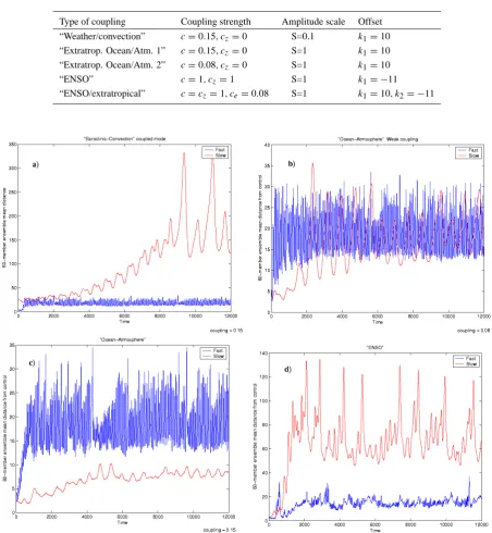
Fig. 1. Evolution of the rms distance of ensemble members for runs corresponding to the first four cases given in Table 1, and random small
initial perturbations.
a suitable approach to filter out the fast modes and extract the slow growing modes in the coupled system.
For the “extratropical ocean-atmosphere” cases, Figs. 1b and 1c, it is clear that the coupling strength modifies their relative amplitude even though we used a unit scaling fac-torS=1. When the coupling is very weak as in Fig. 1c, their amplitudes are nearly the same, but with a somewhat stronger coupling, as in Fig. 1b, the amplitude of the slow “ocean” is considerably reduced, and it becomes a “slave”
Fig. 2. Evolution of the x-component of each of the systems of the coupled model: slow and fast systems for (a) the “weather waves
with convection”, (b) the “ENSO”, and (c) the “Extratropical Atmosphere”, “Tropical Atmosphere” and the “Ocean” sub-systems in the “Tropics-extratropics” coupled model.
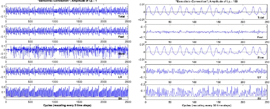
Fig. 3. Left panel: Growth rate of (a) the total BV, (b) fast component, and (c) slow component, (d) LV and (e) SV, (left) using initial
perturbations of 1 for the case of the “weather waves with convection” shown in Fig. 1a, and rescaling every 5 time steps. Right panel: same as left panel but using initial perturbations of amplitude 100 and rescaling intervals of 50 time steps. The results are insensitive to small variations in the amplitude or rescaling interval. Notice that the range is different for the growth rate of the total and the slow
coupling, the two modes evolve with time scales much differ-ent from each other. Therefore, choosing a rescaling interval sufficiently long to allow saturation of the fast mode could reduce its impact on the error growth rate of the coupled sys-tem. In the “ENSO” case (Fig. 1d) we used much stronger coupling (c=1) and coupled the z-component as well, using cz=1. The result is a time-series with a slow mode that shift
regimes every 3 to 12 cycles and a fast mode with more ir-regular behavior (Fig. 2b). Since the coupling is very strong, the saturation time is about the same for the fast and slow so-lutions. Note that even though we used again a scaling factor S=1, in this case the fast solution saturation amplitude is smaller, and the variability lower than in an uncoupled fast system, a result reminiscent to the tropical coupled ENSO response.
In the next two sections we present detailed comparisons of fast and slow growth for the “weather with convection” case, for the “ENSO” case, and for a triply coupled system, in which the tropical atmosphere of ENSO is weakly coupled
with an “extratropical” atmosphere. The other two cases pre-sented in Fig. 1 are less interesting for the following reasons. In the case of Fig. 1b, the slow ocean is driven by the at-mosphere, and provides only a weak feedback, and therefore there are no important slow modes dominating the coupled dynamics. In the case of Fig. 1c, for this configuration of parameters, the two systems are essentially independent, and breeding for the atmosphere and the ocean can be done inde-pendently from each other, rescaling with the corresponding shorter or longer intervals.
3 Separation of the fast and slow modes in the “weather with convection” coupled case
Fig. 4. Same as Fig. 3 but for the coupled “ENSO” system shown in Fig. 1d. The left panel shown the results obtained using a perturbation
size 0.05, and rescaling every 5 steps, and the right panel, results obtained using a perturbation size 20 and rescaling every 50 time steps. The results are insensitive to small variations in the amplitude or rescaling interval.
growth rate (Eq. 1) in Fig. 3, with the left panels correspond-ing to a small amplitudeδ=1 and a short rescaling interval 51t, and the right panels to a large amplitudeδ=100 and a long rescaling period 501t. The top 3 panels correspond to the BVs growth rate computed with the nonlinear model, and the bottom two panels to the LVs and SVs growth rate over the same period, computed with linear tangent model and its adjoint (transpose). In the top three panels we plot the total coupled growth rate (labeled as “total”), the growth rate mea-sured with just the fast variables (“fast”), and the growth rate measured with the slow variables (“slow”). The abscissa is labeled in number of rescaling intervals, but the left and right panels always correspond to the same elapsed physical time. Considering first the left panel, with small amplitudes and short rescaling interval, we see that the growth of the fast “convection” mode is clearly identified, and dominates the total growth. As expected, the growth rate obtained with the linear tangent model (Lyapunov exponent) is also dominated by the fast modes and is essentially identical to that obtained with the BVs. Also as expected, the growth rate of the SVs is considerably larger than that of the LVs. The SV growth rate oscillates with the same frequency as the LV growth rate, but its minimum value is modulated by a frequency associated with the slow modes growth rate (cf. right panel).
The right panels are constructed with parameters chosen to identify the slow “weather waves”, using a large ampli-tude and long rescaling intervals. The top three panels indi-cate that the breeding approach succeeds in isolating the slow modes. The slow growth is apparent when measuring the growth with the slow variables, and it clearly dominates the total growth rate, although during those intervals in which the slow modes decay (growth less than zero), there is a percep-tible influence of the fast modes on the total rate, modulating the rate of decay. In this case, the bottom two panels show that the linear model-based LV and SV growth rates fail to
capture the growth rates of the high amplitude, low frequency “weather waves”, and instead they are still dominated by the high frequency growth of the “convective modes”. It is inter-esting to note that for the longer rescaling, the SVs growth rates are larger but become strongly correlated with the LVs growth rate. This is because the SVs are “optimized” for the rescaling period, and as the optimization period increases, the evolved (final) SVs become parallel to the LVs and grow at a similar rate (e.g. Legras and Vautard, 1997).
These results support the conjecture of Toth and Kalnay (1993, 1996) and Kalnay and Toth (1996), that the selec-tion of rescaling amplitude and frequency could be used to separate fast and slow modes, when the latter have larger amplitudes. It also confirms the results obtained by Lorenz (1996), and is also in agreement with the results of Aurell et al. (1997) and Boffetta et al. (1998). In the next section we tackle more difficult cases in which the scaling factor S is chosen to be unity.
4 Cases of “ENSO” and “ENSO coupled with an extra-tropical atmosphere”
a) “ENSO” case
Fig. 5. Attractors of the 3-component “tropical-extratropical” coupled system corresponding to Fig. 2c. The “tropical ocean” (left) is strongly
coupled to the “tropical atmosphere” (center), which in turn is weakly coupled to the “extratropical atmosphere” (right). The thickness of the arrows indicates the strength of the coupling.
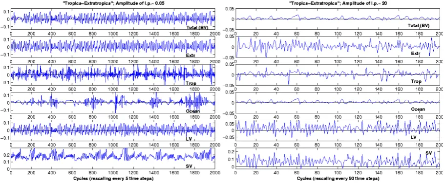
Fig. 6. Same as Fig. 3 and Fig. 4 but for the three component “tropics-extratropics” of Figs. 2c and 5. The rescaling parameters are the same
as in Fig. 4.
total BV growth rate, as it should, since the BVs coincide with LVs in the limit of infinitesimal amplitudes and rescal-ing intervals. For this case even the SV growth rate is dom-inated most of the time by the slowly evolving scales. On the right panels, we see the results obtained using larger am-plitudes (δ=20) and longer rescaling periods (501t). The results for the bred vectors show that the fast growth spurts have been filtered out from the slow and total growth rates, but otherwise there is still a similarity, which is to be ex-pected given the secondary, almost diagnostic role of the at-mosphere in this coupled system. On the other hand, the growth rates for the LVs and SVs are still similar to those ob-tained at low amplitudes and high frequency rescaling (left panels). The spurts of fast growth are still present at the same time, and are only smoothed to the extent that their fre-quency is higher than that of the rescaling, indicating that the linearized models still responds to the same instability char-acteristics. Additional experiments (not shown) indicate that for initial perturbations aboveδ=20 the slow mode has the same temporal structure independently of the rescaling time period, confirming that the slow and total bred vectors have a growth that depends on the stability of the background flow
and not on the details of the parameters used for breeding. b) “Extratropical atmosphere coupled with ENSO” This is the most complex example we will use as illustration of the impact of using different amplitudes and scaling inter-vals. In this case we add an “extratropical atmosphere” which is weakly coupled with the “tropical atmosphere” component of “ENSO”. The equations for this system are as follows:
˙
xe=σ (ye−xe)−ce(Sxt+k1)
˙
ye=rxe−ye−xeze+ce(Syt+k1)
˙
ze=xeye−bze
˙
xt =σ (yt−xt)−c(SX+k2)−ce(Sxe+k1)
˙
yt =rxt−yt−xtzt+c(SY +k2)+ce(Sye+k1)
˙
zt =xtyt−bzt+czZ
˙
X=τ σ (Y−X)−c(xt+k2)
˙
Y =τ rX−τ Y−τ SXZ+c(yt +k2)
˙
Z=τ SXY−τ bZ−czzt
(6)
atmosphere (denoted with a subscripte) weakly coupled to the tropical atmosphere (with a subscriptt), which in turn is strongly coupled to the ocean (upper case variables) as in the ENSO case. The tropical atmosphere and ocean variables are fully coupled with a coupling coefficientc=cz=1, as in
the ENSO case, and the extratropical atmosphere is coupled to the tropical atmosphere with a weak coupling coefficient ce=0.08. Figure 5 shows the shape of the coupled attractor
for each of the components. On the left is the slow ocean, vacillating between a “normal” state which lasts typically 3 to 12 “years”, and an “El Ni˜no” state, which lasts only one “year” (see also Fig. 2c, presenting the x component of the system versus time). In the center is the “tropical ENSO at-mosphere”, faster but strongly coupled to the ocean, as in the ENSO case. On the right is the “extratropical atmosphere” only weakly coupled to the tropical atmosphere, and there-fore looking closer to the classic Lorenz model.
Figure 6 is similar to Fig. 4, but for the tropical-extratropical coupled system. On the left we see that for small amplitudes (δ=0.05) and short rescaling intervals (51t), the growth rate of the extratropical atmosphere domi-nates the total growth rate, as could be expected because the parameters are appropriate for this system. Once again, for small amplitudes and frequent rescalings, the LV growth rate is almost identical to the total growth rate, dominated by the extratropical atmosphere, and the growth rate of the SVs is very large and less variable. For an even shorter rescaling in-terval, the results are similar except for the growth rate of the SVs, which becomes much larger and almost constant, sug-gesting that it cannot discriminate between periods of real growth and decay in the extratropical atmosphere.
On the right, we see that for longer rescaling periods (501t) and larger amplitudes (δ=20), the fast extratropical atmosphere oscillations are essentially completely filtered out, and the ocean growth rate dominates the tropical atmo-sphere, as well as the total growth rate. Unfortunately, the linear approaches of the LV and SV growth, although similar to each other, are strongly influenced by the extratropical so-lutions, and do not provide perturbations appropriate for the longer time scales.
5 Summary and discussion
We have shown that a simple generalization of breeding us-ing amplitudes and rescalus-ing intervals that are physically chosen can be used to separate slow and fast solutions in coupled systems. It should be noted that the results obtained for the BVs and LVs are not sensitive to small variations of the two parameters as long as they are within the range sug-gested by the amplitude and time scales of the coupled solu-tion (Fig. 1). The growth rates for the SVs, by contrast, are considerably more sensitive. The growth rates of the BVs reflect the stability of the basic, evolving flow at the corre-sponding time scales. In addition to their growth rate, this approach yields the bred vectors perturbations appropriate for different types of ensemble forecasts.
The results suggest that for realistic atmospheric models, frequent rescaling (of the order of 10 minutes) and small am-plitudes in the temperatures and other variables could be used to obtain bred perturbations in “storm-scale” models. For large-scale weather forecasting, amplitudes of the order of 1-10m in geopotential heights and intervals of 6–48 h have been already shown to be successful in creating baroclinic initial perturbations. For seasonal and interannual predic-tions, whose skill depends strongly on capturing the evolu-tion of ENSO variability, Cai et al. (2003) have suggested that rescaling intervals of the order of two weeks to a month may isolate coupled model instabilities, and Cai et al. (2003) and Yang et al. (2003) presented results that suggest that this is indeed the case.
Finally, we point out that since there is a relationship be-tween breeding and ensemble Kalman Filtering (e.g. Corazza et al., 2002), our results suggest that for data assimilation in a coupled ocean-atmosphere system, the interval between analyses should be chosen in a similar fashion, allowing enough time for the fast but irrelevant atmospheric oscilla-tions to saturate, and not to overwhelm the slower but impor-tant growth rates of the coupled ENSO instabilities.
Acknowledgements. This research was supported by the NOAA-Office of Global Programs. The authors thank J. Hansen (MIT) for providing the original version of the Lorenz coupled model.
Edited by: A. Osborne Reviewed by: one referee
References
Aurell E., Boffetta, G., Crisanti, A., Paladin, G., and Vulpiani A.: Predictability in the large: an extension of the concept of Lya-punov exponent, J. Phys. A. Math. Gen., 30, 1-26, 1997. Aurell E., Boffetta, G., Crisanti, A., Paladin, G., and Vulpinai, A.:
Predictability in systems with many degrees of freedom, Phys. Rev. E., 52, 2337, 1996.
Bengtsson, L., Schlese, U., Roeckner, E., Latif, M., Barnett, T. P., and Graham, N.: A two-tiered approach to long-range climate forecasting, Science, 261, 1026–1029, 1993.
Boffetta, G., Crisanti, A., Paparella, F., Provenzale, A., and Vulpi-ani, A.: Slow and fast dynamics in coupled systems: A time series analysis view, Physica D., 116, 301–312,1998.
Cai, M., Kalnay, E., Toth, Z.: Bred Vectors of the Zebiak-Cane Model and Their Application to ENSO Predictions, J. Climate, 16, 40–56, 2003.
Corazza, M., Kalnay, E., Patil, D. J., Ott, E., Yorke, J., Szunyogh, I., and Cai, M.: Use of the breeding technique in the estimation of the background error covariance matrix for a quasigeostrophic model, in: AMS Symposium on Observations, Data Assimilation and Probabilistic Prediction, Orlando, Florida, 154–157,2002. Chang, Y., Schubert, S. D., and Suarez, M. J.: Boreal winter
predic-tions with the GEOS-2 GCM: The role of boundary forcing and initial conditions, Quart. J. Roy. Meteor. Soc., 126, 1–29, 2000. Evans, E., Bhatti, N., Kinney, J., Pann, L., Pe˜na, M., Yang, S.-C.,
changes in Lorenz’s model are predictable, Bull. Amer. Meteor. Soc., 85, 520–524, 2004.
Ji, M., Leetmaa, A., and Kousky, V. E.: Coupled model predictions of ENSO during the 1980s and 1990s at the National Centers for Environmental Prediction, J. Climate, 9, 3105–3120, 1996. Kalnay, E.: Atmospheric Modelling, Data Assimilation and
Pre-dictability, Cambridge University Press, 2003.
Kalnay, E., Corazza, M., and Cai, M.: “Are Bred Vectors the same as Lyapunov Vectors?”, extended abstract, http://ams.confex. com/ams/htsearch.cgi, American Meteorological Society meet-ing, Orlando, Florida 13–17 January 2002, 2002.
Kalnay, E. and Toth, Z.:The breeding method, Proc. of the Seminar on Predictability, ECMWF 4–8 September 1995, ECMWF, Shin-field Park, Reading, Berkshire RG29Ax, [email protected], 69–82, 1996.
Legras, B. and Vautard, R.: A guide to Liapunov vectors, Pre-dictability vol I, edited by Palmer, T., ECMWF Seminar, ECMWF, Reading, UK, 135–146, 1997.
Lorenz, E.: Deterministic non-periodic flow, J. Atmos. Sci., 20, 130–141, 1963.
Lorenz, E.: Predictability - A problem partly solved, Proc. on pre-dictability, ECMWF 4–8 September 1995, ECMWF, Shinfield Park, Reading, Berkshire RG29Ax, [email protected], 1–18, 1996.
Palmer, T., and Anderson, D.: Prospects for seasonal forecasting, Quart. J. Roy. Meteor. Soc., 120, 1026–1029, 1994.
Pegion, P., Shubert, S., and Suarez, M.: Boreal winter predictions with the GEOS-2 GCM: The role of the boundary forcing and initial conditions, Quart. J. Roy. Meteor. Soc., 126, 1–29, 2000. Timmermann, A.: The predictability of coupled phenomena, Proc.
of the seminar on predictability of weather and climate, ECMWF 9–13 September 2002, Reading, England, 2002.
Toth, Z. and Kalnay, E.: Ensemble forecasting at NMC: the gener-ation of perturbgener-ations, Bull. Amer. Meteor. Soc., 74, 2317-2330, 1993.
Toth, Z. and Kalnay, E.: Ensemble forecasting at NCEP and the breading method, Mon. Wea. Rev., 125, 3297–3319, 1997. Yang, S.-C., Kalnay, E., and Cai M.: Bred vectors in the NASA
coupled ocean-atmosphere system, Poster presentation, NP8-1WE2P-1657, EGS Geophys. Res. Abstracts, 5, 12 016, 2003. Zebiak, S. and Cane, A.: A model for El Ni˜no-Southern Oscillation,