Anonymization on Refining Partition:
Same Privacy, More Utility
Hong Zhu1, Shengli Tian2, Genyuan Du2, and Meiyi Xie1 1
School of Computer Science and Technology, Huazhong University of Science and Technology Wuhan,Hubei, 430074, P.R.China
2 School of Information Engineering, Xuchang University Xuchang,Henan, 461000, P.R.China
Abstract. In privacy preserving data publishing, to reduce the correlation loss between sensitive attribute (SA) and non-sensitive attributes(NSAs) caused by anonymization methods (such as generalization, anatomy, slicing and randomiza-tion, etc.), the records with sameNSAsvalues should be divided into same blocks to meet the anonymizing demands ofℓ-diversity. However, there are often many blocks (of the initial partition), in which there are more thanℓrecords with dif-ferentSAvalues, and the frequencies of differentSAvalues are uneven. Therefore, anonymization on the initial partition causes more correlation loss. To reduce the correlation loss as far as possible, in this paper, an optimizing model is first pro-posed. Then according to the optimizing model, the refining partition of the ini-tial partition is generated, and anonymization is applied on the refining partition. Although anonymization on refining partition can be used on top of any existing partitioning method to reduce the correlation loss, we demonstrate that a new parti-tioning method tailored for refining partition could further improve data utility. An experimental evaluation shows that our approach could efficiently reduce correla-tion loss.
Keywords:anonymization, refining partition, correlation loss.
1.
Introduction
The anonymization methods, such as generalization [14] [15] [3] [7] [11] [19] anatomy (also called bucketization) [20] [16] [5] slicing [13] [17] and randomization [12] [18] [2], are usually used for privacy preserving data publishing (PPDP). To reduce the correlation loss caused by anonymizing, the records with the sameNSAsvalues should first be divided into blocks to meet the anonymizing demands ofℓ-diversity [1] [14] [15] (i.e., for each block Bthere are at leastℓrecords with differentSAvalues and at most
⌊|B|/ℓ⌋records with the sameSAvalue, otherwise the actualSAvalues of some individ-uals may be disclosed with a certainty higher than1/ℓ). Then, the records of each block in the partition are anonymized, so that theSAvalues appeared in the anonymized block all may be the actualSAvalues of the individuals whose records are in the block.
1.1. Motivation
The optimal partitioning, which puts the records with sameNSAsvalues into the same blocks to meet the anonymizing demands of ℓ-diversity, isNP-hard [7] [11]. So in the (initial) partition there are usually many blocks having more thanℓdifferentSAvalues and uneven frequencies ofSAvalues (i.e., there are more thanℓrecords with differentSA
values and the numbers of the records with differentSAvalues are unequal). Therefore, the average probabilities, which individuals are assigned to their actualSAvalues in the anonymized blocks of these blocks, are smaller. The smaller values mean that there are more correlation loss (less utility), as stated in Section III. If we refine the initial partition, such that the average probabilities of the anonymized blocks of refining partition are max-imized (which are certainly higher than that of the initial partition), then the anonymized data of the refining partition would preserve more utility than that of the initial partition. So a problem arises: anonymizing a dataset such that theSAvalues of individuals should not be inferred with a certainty higher than 1/ℓ while the correlation loss is as less as possible. We believe this is an issue need be addressed.
1.2. Contributions
In this paper, we systematically study anonymization on the refining partition of initial partition in privacy preserving data publishing. Our contributions include the following.
First, we propose an optimizing model for anonymizing a dataset so that the ℓ -diversity is preserved while the correlation loss is as less as possible. According to the model, we propose the approach of anonymizing on the refining partition of initial parti-tion, so that the anonymized data of the refining partition preserves more utility than that of the initial partition.
The second, although the refining partition can be used on top of any existing par-titioning approach, to further reduce the correlation loss, we present a parpar-titioning ap-proach based on the lexicographic andNSAssorting by correlation (betweenSAand each ofNSAs). This approach increases the utility of published data, as it preferentially ensures that a part of theNSAs(more interrelated withSA) values of the records of blocks are the same, while the records of blocks are anonymized, the correlations are retained.
The rest of the paper is organized as follows. Section II briefly reviews related work. Section III presents our problem definition, optimizing model and our purposes. In section IV, we provide our anonymization on refining partition. Section V experimentally eval-uates the effectiveness of our methodology. Section VI gives conclusions and directions for future work.
2.
Related Work
In anonymized data publishing, to prevent the actual sensitive values of individuals from being revealed with high certainty, generalization [14] [15] [3] [7] [11] (and non-homogeneous generalization [19]) transforms the NSAs values of the records of each block into ”less specific” values. Therefore, the information loss caused by generaliza-tion or non-homogeneous generalizageneraliza-tion includes the loss of theNSAsvalues of records, the correlation loss betweenSAandNSAs, and the correlation loss amongNSAs [13]. Anatomy separatesSAfromNSAs by randomly permuting theSAvalues of records in each block [20] [16] [5]. Randomization [12] [18] [2] replaces the SA value of each record in each block with a retention probability pby a value randomly selected from the value-set consisted of theSAvalues of the records within the same block. Thus, there is only correlation loss betweenSAandNSAscaused by anatomy [20][16][5] or random-ization [12] [18], [2], since these methods publish the NSAs values of records in their original forms, there is not the loss of theNSAsvalues of records and the correlation loss amongNSAs. After the records have been partitioned to blocks, slicing [13] and disasso-ciation [17] divide the attributes into columns. Disassodisasso-ciation partitions the attributes into columns based on the items of the values of the attributes. Therefore, the disassociation causes more correlation loss among the attributes of different columns. Slicing partitions the attributes based on the correlation among the attributes, the intersections between the columns and the blocks are buckets, and the tuples in each bucket are randomly permuted. In the buckets withSA, theNSAsvalues of the tuples are generalized. Thus, the informa-tion loss caused by slicing includes the correlainforma-tion loss betweenNSAsandSA, the loss of a part ofNSAsvalues of records, the correlation loss among theseNSAs, and the correlation loss between theseNSAsand the otherNSAs, as theNSAsvalues are generalized.
our method can be used to reduce the information loss caused by all the above anonymiza-tion techniques, since our refining partianonymiza-tion is the local optimal partianonymiza-tion of initial partianonymiza-tion, and anonymization on the refining partition only cause less information loss.
In anonymized data publishing, to reduce the information loss, the records with the sameNSAsvalues should first be divided into blocks with the anonymizing demands ofℓ -diversity. Then, the records of each block in the partition are anonymized. There are many partition methods [19] [20] [5] [6] [22] [21], but none of them meets the demands of the optimizing model, since the partition methods in [19] [5] [6] [22] [21] could not ensure that in each block of the partition the frequencies of differentSAvalues are uniform and the numbers of differentSAvalues is minimized, and the method in [20][8] does not take into account theNSAs values of the records. In addition, all the above methods do not take into account the correlation betweenSAand each ofNSAs. Therefore, as stated in Section III, while the records of the blocks in the partition divided by these methods are anonymized by the above anonymizing techniques, there is more correlation loss.
3.
Problem Definition
Consider a datasetT, in which there are 3 classes of attributes: (1) identifier attributes (IDs), such as name, social security number,IDsare removed in the published table to prevent immediate identification of individuals; (2) sensitive attribute (SA), theSAof in-dividual’s record is the sensitive value of individual; (3) non-sensitive attributes (NSAs), which contain all attributes that do not fall into the previous two categories and which taken together, can potentially identify an individual. Each record inT represents a dis-tinct individual, and eachSAvalue must be distinctively different. We introduce the ’dif-ferent’ in two aspects: (1) ifSAis a nominal attribute that each value in aSAvalue set ofT would be semantic distinguishable, and (2) ifSAis a numerical attribute the difference of any two values are greater than a certain threshold. Otherwise,T should be preprocessed.
3.1. Attack Assumption andℓ-diversity
We assume an attacker may obtain theNSAsand theIDsof any record inT by sources other thanT∗(e.g. a public voters table). LetH be the attacker’s knowledge containing
NSAsvalues andIDsvalues of all known individuals. In the worst case, the attacker may access to theNSAsof every individual, thus by joiningH andT∗onNSAs, recordt∗in T∗ may be linked to an individual (i.e.,t∗ is the anonymized record of the individual’s record).ℓ-diversity principle aims at preventing the attacker from finding an individual’s actualSAvalue with a probability higher than1/ℓ.
Definition 1 (ℓ-diversity principle[14], [15]) LetT∗be an anonymized data table ofT. A records blockB∗ofT∗isℓ-diversity, if there are at leastℓdifferent SA values, which may be the actual SA values of the records in B∗, and the numbers of the different SA values are all not more than⌊|B∗|/ℓ⌋.T∗ isℓ-diversity, if all the blocks of T∗ areℓ -diversity.
3.2. Our Goal
While the original blockBis anonymized (to generateB∗), the anonymization methods all destroy the correlations. In addition, as stated in Section II, some methods also lose other information, since theNSAs values of records have been dealt. AsH may be ob-tained from public resources, data accepter may prefer to care the correlations between
SAandNSAs.
Therefore, our goal is to acquire a local optimal partition of T such that the anonymized table T∗, which is consisted of the anonymized blocks (of the blocks of the partition), meets the following two conditions:
(1)ℓ-diversity principle is satisfied.
(2) the correlation loss betweenSAandNSAsis as less as possible.
3.3. Problem Definition and Optimizing Model
Consider any anonymized blockB∗inT∗(withℓ-diversity). LetBbe the original block ofB∗,t1, t2, . . . , tnbe the records ofB(n=|B|)andt∗1, t∗2, . . . , t∗nbe the corresponding
anonymized records inB∗. Assume theSAvalue-set (multiset) composed of theSAvalues appeared inBareS ={s1:c1, s2:c2, . . . , sm:cm};mis the number of differentSA
values,(m ≥ ℓ);ci is the number of the records with theSAvaluesi (inB). For each
ci(1≤i≤m),ci≤ ⌊|B|/ℓ⌋, (i.e.,ci/|B| ≤1/ℓ), sinceT∗isℓ-diversity.
Property 1 the mean value of the probabilities, which the records (t∗) inB∗are assigned to their actual SA values (t[SA]), isp(t∗, t[SA]) =∑mi=1(ci
n)
2
≤1
ℓ .
Proof. p(t∗, t[SA]) = 1n∑ni=1p(t∗i, ti[SA]) = 1n(c1×cn1 +c2×cn2
+. . .+cm×cnm) = n1
∑m i=1
ci×ci
n =
∑m i=1(
ci n)
2.
∀t∗i ∈B∗,1≤i≤n, p(ti∗, ti[SA])≤1ℓ, asB∗isℓ-diversity.
Thus,1n∑ni=1p(ti∗, ti[SA])≤ 1ℓ.
Therefore,p(t∗, t[SA]) =∑mi=1(cin)2≤1ℓ.
The precise correspondences (such as an actualSAvalue is assigned to an individual inB) are all converted to imprecise correspondences (such asmdifferentSAvalues are as-signed to the individual inB∗) by anonymization methods. Thus, the smaller the value of mis, the more precise correspondence is (i.e., the less correlation loss is), and the higher the probability value is, the more precise correspondence is (i.e., the less correlation loss is). However,ℓis the minimal value ofmand1/ℓis the maximal value of the probability, due toℓ-diversity.
Therefore, for each blockB∗ ofT∗, the bigger the value of the average probability p(t∗, t[SA])is, the less correlation loss is (i.e., the more precise correspondence is). In addition, as∑mi=1ci=n,
p(t∗, t[SA]) =
m
∑
i=1 (ci
n) 2
= c
2
1+c22+. . .+c2m
(c1+c2+. . .+cm)2
Having computed the partial derivatives ofp(t∗, t[SA])forc1, c2, . . . , cm, we acquire
the conditional extreme value, i.e., while the values ofc1, c2, . . . , cmare the same andm
isℓ, the value ofp(t∗, t[SA])is maximized, the maximal value is1/ℓ.
However, the optimal partition that put the records with the sameNSAs values into the same blocks (with the demands ofℓ-diversity) isNP-hard [7] [11]. Thus, there are often many blocks having more SAvalues and uneven frequencies ofSAvalues, such that thep(t∗, t[SA])values of the anonymized blocks of these blocks are lower. To gen-erateℓ-diverseT∗(ofT) so that the correlation loss is as less as possible, we propose an optimizing model.
Definition 2 (Optimizing model) LetT∗ be an anonymized data table ofT. For each blockB∗ ofT∗ (letB∗be the anonymized block ofB), if the following conditions (1), (2), (3) and (4) are satisfied, and thep(t∗, t[SA])is maximized, thenT∗is an optimizing
ℓ-diverse anonymized data table.
(1) A part of NSAs (having higher correlation with SA) of the records (ofB) are the same values;
(2)ci/n≤1/ℓ,1≤i≤m; (3)∑mi=1ci=n;
(4)ℓ≤m≤n.
In the best case, theNSAsof the records ofBshould have the same values. While the records with differentNSAsvalues must be merged to the block for meeting the demands ofℓ-diversity, we should ensure that a part ofNSAs(having higher correlation withSA) of the records ofB are the same values, as stated in the condition (1), i.e., we should as less as possible break the correlations (betweenNSAsandSAinT) inB∗. In addition, the conditions (2), (3) and (4) ensure thatB∗isℓ-diversity.
4.
Anonymization on Refining Partition
We follow the following framework. (1) The records are divided into blocks with the anonymizing demands ofℓ-diversity. (2) Based on the optimizing model, the initial parti-tion is refined. (3) The records of each block of the refining partiparti-tion are anonymized by the methods such as anatomy, generalization or slicing, etc.
4.1. Initial Partitioning
To preferentially retain the correlations between a part ofNSAs(having more interrelated withSA) andSA, which further increases the data utility of anonymized table, we also propose a partitioning approach based on the lexicographic andNSAssorting by the cor-relation betweenNSAandSA.
1) Computing correlation
v11, v12, . . . , v1d1, andSAwith value-set of data tables1, s2, . . . , sd. Their sizes of
value-sets are thusd1andd, respectively. The mean-square contingency coefficient betweenA1 andSAis defined as:
ϕ2(A1,SA) =
1
min{d1, d} −1 ×
d1
∑
i=1
d
∑
j=1
(fij−fi.f.j)2
fi.f.j
.
Here,fi. andf.j are the fraction of occurrences ofv1i andsj in the data,
respec-tively. Thefij is the fraction of co-occurrences ofv1i andsj in the data. Thefi. and
f.j are the marginal totals of fij : fi. =
∑d
j=1fij andf.j =
∑d1
i=1fij . Obviously, 0≤ϕ2(A
1,SA)≤1. The higher the value ofϕ2(A1,SA)is, the more related betweenA1 andSAare.
2) Partitioning
Having computed the correlations forSA and all NSAs of data table T, the NSAs
of T are sorted by their correlations in descending. Then, the records ofT are sorted by lexicographic NSAs order. The records are partitioned in a top-down fashion. First, we consider attributeA1, which the value ofϕ2(A
1,SA)is the biggest among allNSAs (A1, A2, . . . , A|N SAs|), and put records with the sameA1value in the same block. This results in a set of blocksB1, B2, . . . , Bm, (assumed1=m). However, some blocks may not satisfy the anonymizing demands ofℓ-diversity. For each such blockBj, we random
find a neighboring blockBx(eitherBj−1orBj+1), and mergeBxwithBj. After we have
done withA1, we recursively partition the resulting blocks using the next attribute in order (i.e.,A2). In some blocks, the records may have differentA1 values (due to merging). For such blocks, we do not attempt to further decompose them recursively using another attribute. The partitioning strategy is repeated until all blocks are finalized or there are no more attributes that can be used for recursive partitioning. The detailed process is shown in Algorithm 1.
Each block of the initial partition generated by Algorithm 1 satisfies the anonymiz-ing demands of ℓ-diversity. As shown in line 1 of Algorithm 1, B is divided into B1,B2,. . .,Bmusing the current N SA(i.e.,Ai). For each Bj which do not meet the
anonymizing demands ofℓ-diversity, a neighboring block of Bj (i.e.,Bx) is merged to
Bj. At worst,B1, B2, . . . , Bmare all merged to the block (i.e.,B), andB satisfies the
anonymizing demands ofℓ-diversity (as stated by the Precondition of Algorithm 1). Thus, at the end of the iterations (line 2∼5), the sub-blocks ofBmust meet the anonymizing demands ofℓ-diversity. Some sub-blocks ofB, which have differentAi values (due to
merging), are output. In some sub-blocks ofB, the records have the sameAi values. If
i=|N SAs|, output such sub-blocks. Otherwise, the partition attempts to further decom-pose them until all blocks are finalized or there are no more attributes that can be used for recursive partitioning. Therefore, as stated above, each block of the initial partition generated by Algorithm 1 satisfies the anonymizing demands ofℓ-diversity.
4.2. Refining Partitioning and Anonymizing
To maximize the mean probabilities which individuals are assigned to their actual SA
Algorithm 1Partitioning (B, ℓ, Ai)
Precondition:Bsatisfies the anonymizing demands ofℓ-diversity.
Input: a set of recordsB, parameter inℓ-diversity, attributeAiis used for partitioning.
Output: sub-blocks ofB.
1: PartitionBintoB1, B2, . . . , BmusingAi //Assume|Ai|=m.
2: foreachBjwhich do not meet the anonymizing demands ofℓ-diversitydo 3: Random findBxas a neighboring block ofBj
//Bxmay beBj−1orBj+1 4: MergeBjandBx
5: end for
6: foreachBjdo
7: if (∃ta, tb∈Bj∧ta[Ai]̸=tb[Ai])∨(Ai=A|N SAs|)then 8: Output(Bj) //Output the blockBj
9: else
10: Partitioning (Bj, ℓ, Ai+1) // recursive call 11: end if
12: end for
and uniform. Therefore, we refine the initial partition such that any block of the refining partition is composed ofℓrecords with mutual differentSAvalues. The residual records of the neighbor block of initial partition are merged to form a sub-block (composed of ℓ records with differentSAvalues) of refining partition. In this case, thep(t∗, s)value of each anonymized block of the block in the refining partition is the maximum value (i.e., 1/ℓ). Finally, the last residual records (which the number of records with different
SAvalues is less thanℓ) are respectively inserted into the corresponding sub-blocks of the refining partition. The detailed process is shown in Algorithm 2.
Property 2 In Algorithm 2, for eachBi(1≤i≤m), at the end of the iterations (line 4 ∼8), the number of nonempty buckets is|Bi|modℓ, and there is only one record in each nonempty bucket.
Proof. For each iteration,ℓrecords with the mutual differentSAvalues are removed from theℓlargest nonempty buckets (i.e., in each bucket, only one record is random removed). So the iterations all are executed⌊|Bi|/ℓ⌋times, denoted asI1,I2,. . .,I⌊|Bi|/ℓ⌋,
respec-tively.
Otherwise, we assume the iterations all are executed⌊|Bi|/ℓ⌋ −1times. At the end of the iterations, the number of the nonempty buckets is at mostℓ-1, (otherwise, the iterations could not have terminated). Then there is a set of nonempty buckets with at least2records (as the number of the residual records (termedx) isℓ ≤x <2ℓand the number of the nonempty buckets is at mostℓ−1).
Let a residual buckets (rb) have at least2records. Before iterationI⌊|Bi|/ℓ⌋−1starts, at most ℓ-1 buckets (including rb) have at least 3 records (otherwise, there would be ℓ nonempty buckets afterI⌊|Bi|/ℓ⌋−1, contradicting the fact thatI⌊|Bi|/ℓ⌋−1 is the last iteration). Thus,rbloses a record forI⌊|Bi|/ℓ⌋−1, meaning that, beforeI⌊|Bi|/ℓ⌋−1, therb has at least3records.
Similarly, before I⌊|Bi|/ℓ⌋−2, at most ℓ −1 buckets (including rb) have at least 4
contradicting our earlier analysis). Thus,rbloses a record forI⌊|Bi|/ℓ⌋−2, meaning that, beforeI⌊|Bi|/ℓ⌋−2, therbhas at least4records.
Carrying out the same discussion to the other iterations, we arrive at a fact that therb
has at least⌊|Bi|/ℓ⌋+ 2(i.e.,⌊|Bi|/ℓ⌋+ 1) records beforeI1. This fact violates that there are at most|Bi|/ℓrecords with the sameSAvalues inBi.
For the similarly reason, we could get the fact, which there are at least⌊|Bi|/ℓ⌋+ 1 records in a bucket beforeI1, and this fact violates that there are at most⌊|Bi|/ℓ⌋records with the sameSAvalues inBi, if the iterations are executed less than⌊|Bi|/ℓ⌋times. Thus,
when the iterations terminate, it must have been executed⌊|Bi|/ℓ⌋times. So the number of the residual records is|Bi|modℓ. The residual records must have mutual differentSA
values (i.e., each non residual bucket has only one residual record.), otherwise, assume there are two residual records having the same SA values, using the above similarly analysis, beforeI1, there must be⌊|Bi|/ℓ⌋+ 1records have the sameSAvalues. This fact violates that there are at most|Bi|/ℓrecords with the sameSAvalues inBi.
Property 3 In Algorithm 2, for eachBi(1≤i≤m), at the end of the iterations (line 4 ∼8),⌊|Bi|/ℓ⌋blocks (i.e., Sub B[i1], Sub B[i2],. . ., Sub B[i⌊|Bi|/ℓ⌋]) are generated. If |Bi|modℓis not zero, then for each residual record (t), there is a Sub B[ic], (1 ≤c ≤ ⌊|Bi|/ℓ⌋), in which the SA values of the records are different with t[SA].
Proof. Assume, on the contrary, there is a residual record (t), for ∀ Sub B[ic], (1 ≤
c ≤ ⌊|Bi|/ℓ⌋),∃t′ ∈Sub B[ic]∧t[SA]=t′[SA]. Then, the number of the records
(hav-ing the sameSAvalue witht) is⌊|Bi|/ℓ⌋+ 1. This fact violates that there are at most
⌊|Bi|/ℓ⌋records with the sameSAvalues inBi. Thus, for each residual record (t), there
is a Sub B[ic], (1≤c≤ ⌊|Bi|/ℓ⌋), in which theSAvalues of the records andtare mutual
different.
Property 4 In Algorithm 2, for each record t in R B (line 16), there is a block Sub B[j] (1 ≤j ≤count), which t[SA] and the SA values of the records in Sub B[j] are mutual different.
Proof. For∀t ∈R B,∃Bi(1 ≤ i ≤ m)∧t ∈ Bi, as t is a residual record ofBi (at
the end of the iterations (line4∼8)). By Property 3, we know that there is a Sub B[ic],
(1 ≤c≤ ⌊|Bi|/ℓ⌋), in which theSAvalues of the records are different witht. Thus, the Sub B[ic] would be as Sub B[j] (1≤j≤count).
Here we propose a hypothesis. LetT3∗be an anonymized table, which is generated by the following two steps.
First, for eachBi,(1≤i≤m), if|Bi|modℓis not zero, then all the residual records
are inserted into their corresponding sub-blocks (since as stated in Property 3, for each residual record (t), there is a Sub B[ic], (1≤c≤ ⌊|Bi|/ℓ⌋), in which theSAvalues of the
records are different witht[SA]). Let(p(t∗, s))′be the mean probability, which individuals are assigned to their actualSAvalues in the anonymized blocks of the sub-blocks ofBi.
As stated in Property 1,p(t∗, s)is the mean probability that individuals are assigned to their actual SAvalues in the anonymized blocks of Bi. Then,p(t∗, s) ≤ p(t∗, s)′, as
shown in Property 5.
Algorithm 2Refining-partition-anonymizing (T, ℓ)
Precondition:(1)T satisfies the anonymizing demands ofℓ-diversity; (2) the records inT have been sorted by lexicographical andNSAsattributes (A1, A2, . . . , A|N SAs|) ordering.
Input: a data tableT, the parameter inℓ-diversity.
Output: anonymized tableT∗.
1: Partitioning (T, ℓ, A1) // also by others partition approach // LetB1, B2, . . . , Bmbe the blocks of initial Partition // Let Sub B be an array consisted of sub-blocks // Let count be counter, which initial value is 0 // R-B is used to retain residual records, which // initial value isΦ.
2: foreachBido
3: Hash the records inBiby theirSAvalues to buckets //each bucket perSAvalue; at leastℓnon-empty hash
//buckets due to at leastℓrecords with the differentSAvalues inBi 4: while(there are at leastℓnon-empty hash buckets)do
5: Takeℓlargest non-empty bucketsb1, b2, . . . , bℓ 6: Set count= count+1
7: Set Sub B[count]=Φ// i.e., Sub B[count]is empty
8: Random remove a record of eachbjto Sub B[count] //1≤j≤ℓ 9: end while
10: Remove the record of each nonempty bucket to R B //only|Bi|modℓnonempty buckets, each nonempty //bucket per record, as shown in Property 2
11: whilethere are at leastℓrecords with differentSAvalues in R Bdo
12: Set count= count+1
13: Set Sub B[count]=Φ// i.e., Sub B[count]is empty
14: Remove theseℓrecords of neighbor blocks to Sub B[count] 15: end while
16: end for
17: ifR B is non emptythen
18: for For eachtin R Bdo
19: Find a Sub B[j] such that
∃Bi(t∈Bi)∧ ∃Sub B[j](Sub B[j]⊆Bi)∧ ∀t′∈Sub B[j](t′[SA]̸=t[SA]), 1≤i≤m,1≤j≤count
// as shown in Property 4 20: Removetto Sub B[j] 21: end for
22: end if
is generated by anonymizing on refining partition. Then,T1∗,T2∗andT3∗satisfy Property 6.
Property 5 p(t∗, s)≤p(t∗, s)′
Proof. As stated in Property 1, S = {s1 : c1, s2 : c2, . . . , sd : cd},dis the number
of differentSAvalues inBi,cj is the number of the records havingsj asSAvalue, and
p(t∗, s) =∑dj=1( cj |Bi|)
2. There are following two cases.
Case 1 (the frequencies of theSAvalues inBiare uneven): assumecb(1≤b≤d)is
biggest amongc1, c2, . . . , cd. Thencb ≤ ⌊|Bi|/ℓ⌋(as there are at most⌊|Bi|/ℓ⌋records
with the sameSAvalues inBi, andcdmust be integer). Thus,
∑d j=1(
cj |Bi|)
2< 1
|Bi|×
∑|Bi| cb |Bi| =
cb |Bi|≤
⌊|Bi|/ℓ⌋ |Bi| .
Therefore, the average probability ofBiisp(t∗, s)< ⌊| Bi|/ℓ⌋
|Bi| . But the average
prob-ability, which these individuals are assigned to their actualSAvalues in the anonymized blocks of Sub B[i1], Sub B[i2],. . .and Sub B[i⌊|Bi|/ℓ⌋] is
p(t∗, s)′= |B1
i|
∑⌊|Bi|/ℓ⌋ x=1
∑|Sub B[ix]|
1
1
|Sub B[ix]|= ⌊|Bi|/ℓ⌋
|Bi| .
Thus,p(t∗, s)< p(t∗, s)′.
Case 2 (the frequencies of theSAvalues inBiare uniform): then thec1, c2, . . . , cdare
equal (denoted byc), and|Bi|=c×dandd≥ℓandc/|Bi| ≤1/ℓ.
The mean probability, which the individuals are assigned to their actualSAvalues in the anonymized block ofBi, is
p(t∗, s) =∑dj=1(|Bcj
i|)
2=∑d j=1(
c |Bi|)
2=d×c |Bi|×
c |Bi| =
c |Bi|=
1
d.
The mean probability which these individuals are assigned to their actualSAvalues in the anonymized blocks of Sub B[i1], Sub B[i2],. . .and Sub B[i⌊|Bi|/ℓ⌋] is
p(t∗, s)′ = |B1
i|
∑⌊|Bi|/ℓ⌋ x=1
∑|Sub B[ix]|
1
1
|Sub B[ix]| =
⌊|Bi|/ℓ⌋ |Bi| =
⌊(d×c)/ℓ⌋
d×c ≥
⌊(d×c)/d⌋
d×c =
c d×c =
c d×c =
1
d.
Thus,p(t∗, s)≤p(t∗, s)′.
According to Case 1 and Case 2,p(t∗, s)≤p(t∗, s)′.
Property 6 The average probabilities, which individuals are assigned to their actual SA value inT1∗, is more than that ofT3∗andT2∗.
Proof. According to Property 5, for eachBi,(1≤i≤m),p(t∗, s)≤p(t∗, s)′. Therefore,
the average probability, which individuals are assigned to their actualSAvalue inT3∗, is more than that ofT2∗.
In the following, we prove that the average probability ofT1∗is more than that ofT3∗. Assume at the end of line 14 of Algorithm 2, there aret1, t2, . . . , tp in R B. Among
them, assumeta1, ta2, . . . , taz(z≤p)be a part of residual records ofBi, (1≤i≤m).
z≤y≤ℓ−1, as some residual records ofBiand some residual records of the neighbor
blocks ofBimay be merged to a new sub-block of refining partition (line10∼13).
At the end of the iterations (line 4 ∼ 8), let the sub blocks ofBi be Sub B[i1],
Sub B[i2],. . ., Sub B[i⌊|Bi|/ℓ⌋]. At the end of the iterations (line16∼18), i.e.,ta1,ta2,
. . .,taz have been inserted into some sub blocks (by Property 4) ofBi. Then the average
probability, which the individuals (whose records are inBi) are assigned to their actual SAvalues inT1∗, is:
p(t∗, s)′′= |B1
i|(
(y−z)
ℓ +
∑⌊|Bi|/ℓ⌋ x=1
∑|Sub B[ix]| j=1
1
|Sub B[ix]|) =
⌊|Bi|/ℓ⌋ |Bi| +
(y−z)
|Bi| .
But the average probability, which the individuals (whose records are in Bi) are
assigned to their actualSAvalues inT3∗, is p(t∗, s)′= |Bi1|∑⌊|Bi|/ℓ⌋
x=1
∑|Sub B[ix]|
1
1
|Sub B[ix]|=
⌊|Bi|/ℓ⌋ |Bi| .
Asz≤y, y|Bi−z| ≥0. Thus,p(t∗, s)′≤p(t∗, s)′′.
In addition, as stated above, the mean probability ofT3∗is more than that ofT2∗. Thus, the mean probability ofT1∗is more than that ofT2∗.
4.3. The Analysis of Anonymization on Refining Partition
1) Security Analysis
Assume that theT∗ is generated by the Algorithm 2 based on slicing (anatomy or generalization, etc.). Since in each block ofT∗there are at leastℓdifferentSAvalues and the numbers of the differentSAvalues are the same value1, the probabilities, which the individuals (linked to the anonymized block by theirNSAsvalues) are assigned to their actualSAvalues, all are not more than1/ℓ. Therefore,T∗isℓ-diversity.
2) Utility Analysis
(1)T∗retains more correlations
In this section, we illustrate that theT∗ generated by our approach has more data utility from the following two aspects.
Property 7 The correlations between NSA (having more interrelated with SA) and SA are retained inT∗.
Proof. Assume that theNSAssorting by the correlations (betweenNSAsandSAinT) in ascending areA1, . . . , Ay, , A|N SAs|. Lety(1≤ y ≤ |N SAs|)be the maximum value,
such that in each blocks ofT∗the records have the sameAyvalue. Letvx1, vx2, . . . , vxdx
be the set which is consisted of the Ax values in T, and dx be the size of such set.
s1, s2, . . . , sdis consisted of theSAvalues inT, anddbe the size of such set.
For eachx, (1 ≤x≤y), in each block ofT∗, the records have the sameAxvalue,
due to our partition approach. Thus, each record ofT∗has the sameAxvalue with that
the records inT∗ retain their original forms inT. Therefore, for eachvxi (1≤i≤dx),
the frequency ofvxivalue inT∗(i.e.,fxi∗.) is equal tofxi.(i.e., the frequency ofvxivalue
inT).
The frequency ofSAvalue inT∗is equal to that of the homologousSAvalues inT, as the above anonymizing methods do not destroy the frequency ofSAvalue ofT. Thus, for eachsj(1≤j≤d), the frequency ofsjinT∗is equal to that of inT, i.e.,f.j∗ is equal
tof.j.
In addition, letfxi.j be the co-occurrences ofvxi andsj inT, i.e., there are fxi.j
records, whichAxvalues arevxi andSAvalues aresj. Based on our partition approach
we know that the records are divided intofxi.jsub-blocks of the refining partition. In each
sub-block, there only is one record has theSAvaluesj, as theSAvalues of the records in
each sub-block are mutual different. Since theAxvalues of the records in each sub-block
are the same value, and the Ax values of the records of fxi.j sub-blocks are the same
value, in the anonymized sub-blocks of thefxi.jsub-blocks (inT∗), theAxvalues of the
records remainvxi. Therefore, while the co-occurrences ofvxi andsj are calculated in
T∗, there only are thefxi.j blocks having the occurrences, and there only is one
co-occurrence in each block. Therefore, the co-co-occurrences ofvxi andsj inT∗(i.e.,fx∗i.j)
remainfxi.j, which is the co-occurrences ofvxiandsjinT.
In conclusion, each parameter ofϕ2(A
x, SA)calculated inT∗is the same as that is
calculated inT. Thus, theϕ2(A
x, SA)value in theT∗is the same as that is calculated in
T, since all the values of the parameters of the formulaϕ2(A
x, SA)computed inT are
the same as that are calculated inT∗. As1 ≤x≤y, theNSA(having more interrelated withSA) andSAare retained inT∗.
Our approach increases the utility ofT∗, as the correlations between a part of the
NSAs(having more interrelated withSA) andSAare retained inT∗. (2)T∗has lower bound ofRE
The reconstruction error [20] [13] [12] [18] [2] (denoted byRE) often is used to mea-sure the information loss (betweenNSAsandSA) of published table caused by selected anonymized technique, such as slicing, anatomy and generalization, etc.
As stated in [1], the actualNSAs values of the records of published table are easy to be acquired, in this section while the RE of the anonymized table is computed, the information loss ofNSAs values of records may not be taken into account, even if the anonymized table is generated by generalization. For illustration purposes, and to show theREof the anonymized table generated by our method (i.e., refining partitioning and anonymizing), assume that T∗ is generated by anatomy, as all theNSAs values of the records inT∗retain original forms. We demonstrate thatT∗has lower bound ofRE, as shown in Property 8.
For each blockB∗ofT∗(B is the original block ofB∗), letSBbe theSAvalue-set
composed of all the SAvalues appeared inB. For each individual (t) whose record is linked toB∗by theNSAsvalues oft, theREoftis the probability that all the values in SB(which are not the actualSAvalue oft) are assigned tot.
Property 8 T∗has lower bound of RE.
Case 1 (r = 0): by Algorithm 2 we know that each block BinT∗ hasℓindividual records, and their SA values are mutual different. Therefore, the probability that each individual (t) is assigned to the actualSAvalue of tis1/ℓ. So theREof tis1−1/ℓ. Thus theREof all individual records inT∗are
∑n
1(1− 1
ℓ) =n×(1−
1
ℓ).
Case 2(r ̸= 0): at the end of line 14 of Algorithm 2, there are n−rindividual records which have been divided into blocks, in which there are exactly ℓ individual records having mutual differentSAvalues. According to the analysis of Case 1, the total
REof these records is
(n−r)×(1−1/ℓ).
Next, we show after inserting a residual recordtto a block, in which theSAvalues of the records and theSAvalue oftare mutual different (as shown in line16 ∼ 19of Algorithm 2), the overallREincreases by 1. Without loss of generality, assume thattis inserted to a block (with d records). Before the insertion, following the derivation of Case 1, the totalREof the records in the block isd×(1−1d). After the insertion, the totalRE
becomes(d+ 1)×(1−d+11 ), so that the totalREof the records in the block increases by:
(d+ 1)×(1−d+11 )−d×(1−1d) = 1.
As mentioned earlier, before the insertion step starts, the totalREequals(n−r)× (1−1
ℓ). Therefore, after insertion allrresidual records, the totalREbecomes:
(n−r)×(1−1
ℓ) +r=n×(1−
1
ℓ)×(1 + r n×(ℓ−1)).
That is greater than the lower boundn×(1−1/ℓ)by a factor of(1 + (n×(rl−ℓ))). GenerallyTusually is a large data table, the number of the residual records is far less thann, sor≪n×(ℓ−1), i.e.,1 + r
n×(ℓ−1) ≈1.
Therefore, in this case, the totalREof the individual records inT∗is extremely close to the lower bound.
Actually the higher the probabilities that the individuals are assigned to their actualSA
values are, the lower bound ofREis. In our approach, the probabilities that individuals are assigned to their actual SAvalues are increased, as stated in Property 5. Thus,T∗ has lower bound ofRE. In the same time, the lower bound of reconstruction error ofT∗ illustrates that our approach is valid to increase the data utility of the published data.
(3) Cost Analysis
Before we apply Algorithm 2, we need compute the correlations betweenNSAsand
SA, then rearrange the order ofNSAsand sort the records for Algorithm 1. Suppose the number of attributes in NSAs isb, each partition defined by the first attribute of NSAs
recursively is repartitioned up tob times. In the worst case, the cost of the partition is
comparing with|T|. Therefore, the overall cost of anonymization on refining partition is O(|T| ×log(|T|)).
5.
Experiments
All of the experiments are conducted inDelphi7.0and are run on anIntel Core 2.8 GHz
machine and 2GB RAMwithWindows XP. We use theAdultdataset from theUC Irvine
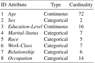
machine learning repository [10], which is comprised of data collected fromUS census. The dataset has been used in several literatures [14] [15] [11] [19] [13] for privacy pre-serving data publication. Records with missing values are eliminated, and there are 30718 valid records used in our experiments. TheAdult dataset contains 15 attributes in total. We randomly project 8 attributes (Age,Sex,Education-Level,Marital-Status,Race, Work-lass,Country,Occupation) from the original table as the experimental dataset, and the attributes forAdultdataset in our experiments are described in TABLE I. TheOccupation
is taken asSAand the other attributes are taken asNSAs.
Table 1.Description of the dataset
ID Attribute Type Cardinality
1 Age Continuous 72
2 Sex Categorical 2
3 Education-LevelContinuous 16 4 Marital-Status Categorical 7
5 Race Categorical 5
6 Work-Class Categorical 7 7 Relationship Categorical 6 8 Occupation Categorical 14
In this section, we illustrate that theT∗generated by our method has less correspon-dences (betweenNSAsvalues andSAvalues of records) loss. If the correspondences (be-tweenNSAsvalues andSAvalues of records) inT∗are not damaged, then for eachNSA
(Ax) ofNSAs, there is not the correlation (betweenAxandSA) loss, since the value of
ϕ2(A
x,SA)inT is equal to the value ofϕ2(Ax,SA)inT∗. Therefore, the less the
corre-spondence loss is, the less correlation loss is (the more data utility ofT∗is).
The count queries [20] [12] [18] [2] usually are used to measure the correspondences loss of anonymized table. However, the methods only select a small part of records of
T as query predicates. Thus, the count queries do not accurately measure the loss. To accurately measure the correspondences loss, the approach of [9] is used in this paper, all the records ofT are taken as query predicates to query in anonymized tableT∗. Assume Sis theSAvalue-set composed of theSAvalues of the records inT. For each record (t) in T, letStbe theSAvalue-set composed ofSAvalues of the records having the sameNSAs
values witht. Obviously, for eachsinS−St, inT there is not the record, which has
theNSAsvaluest[NSAs] and has theSAvalues. But inT∗the values inS−Stmay be
SAof the records of T. Thus, the probability, which the values inS −St may be the SAvalue oft∗(inT∗), is taken as the normalized correspondences loss penalty (NLP) of the recordt(as shown in Definition 3). The minimum value ofNLP(t∗) is zero, and the correspondences loss is zero when recordt∗is generated fromt. TheGLPis a normalized version ofNLP. The smaller the value ofNLP(t∗) is, the better data utility is achieved, so do asGLP(T∗). In this paper, theGLPis used to measure the correspondences loss of anonymized table generated by different anonymization approaches.
Definition 3 (GLP [8],[9]]) LetT∗be an anonymized data table ofT. Assume thatS is theSAvalue-set ofT. Lett[SA] be the SA value oft, andStbe a SA value-set consisted of the SA values of the records having the same NSAs values witht, i.e.,∀t∈T,∃St(t[SA]∈
St)∀t′ ∈T(t[NSAs] = t′[NSAs]→ t′[SA] ∈St). The normalized correspondences loss penalty that generate recordt∗ fromt(tandt∗belong to the same individual) is NLP. NLP(t∗)=∑s∈(S−St)Pr(t∗[SA] =s). The GLP is a normalized version of the NLP.
In the following discussion, our method anonymization on refining partition is de-noted by ARP, the anonymization on the initial partition is denoted by AIP. We select bucketization as the anonymization approach ofARPandAIP, since we only to compare the correlation loss of anonymized data, as stated in our goal (of Section III). Since the partition of anatomy [20] (denoted byAT) often is used in other methods [19] [13] [18], we compare theGLPofATwithARP. In addition, since non-homogeneous generalization (denoted byNG) also is used to reduce the information loss caused by generalization, as stated in literature [19], we compare theGLPofNGwithARP. Without loss generality, we also generate the partition ofNGby Algorithm 1.
Our experiments demonstrate that the execution-time and correspondences loss of
ARPcomparing withAIP,NGandAT, when privacy level (ℓ), the size (n) of the dataset and the size (d) ofNSAsof dataset are varied.
5.1. Varying Privacy Level
1) Experimental results
In this experiments, we set the size of the dataset n=20 thousands. With privacy level ℓincrease, the execution time and theGLPof four methods are shown in Fig. 1 and Fig. 2.
(1) Withℓincrease, the execution times of four approaches are increasing, as shown in Fig. 1. Among them, the execution time ofNGis always maximal. The execution time ofARPis more than that ofATandAIP, and there are fluctuations in the execution time ofAT.
(2) Withℓincrease, theGLPof four approaches are increasing, as shown in Fig. 2. Among them, theGLPofATis always maximal. TheGLPofARPandNGare almost the same in statistical sense, and their values are always minimal.
2) The analysis of the experimental results
(1) For the experimental result (1), comparing withARPandNG, the anonymization of AIP is directly applied on the initial partition, so AIPspends less time than that of
0.25 0.3 0.35 0.4 0.45 0.5 0.55 0.6 0.65 0.7 0.75
l ( l−diversity)
Time (
Second)
l=3 l=5 l=7 l=10
ARP AIP AT NG
Fig. 1.Execution time; varyingℓ
the partition approach ofAIP need spend more time on computing the information of
SAvalues of blocks (for judging the demands ofℓ-diversity), the approach of AT only counts the numbers of records of blocks (for judging the demands ofℓ-diversity), as the
SAvalues of the records of each block ofATare mutual different. The fluctuations in the execution time ofATis because of the randomization of the partition, and withℓincrease, the execution time ofATis increasing, since it need spend more time on partitioning. With ℓincrease, the numbers of the records in the blocks of initial partition are increasing, so
AIPspends more time on computing the information ofSAvalues of blocks (for judging the demands ofℓ-diversity), and comparing withAIP,ARPandNGneed spend more time to anonymize records. Therefore, withℓincrease, the execution time ofAIP,ARPandNG
are increasing.
(2) For the experimental result (2), in each block ofAT, theSAvalues of records are mutual different, and theNSAs values of records may be different sinceAT is not care about theNSAs values of records. Thus, the GLP ofAT is always maximal. Although the records with same NSAs values are divided into same blocks ofAIP, the numbers of differentSAvalues in the blocks ofAIPare always more thanℓand the records with differentNSAsvalues would be in the same block due to neighbor block merging (to meet the demands ofℓ-diversity). Therefore, although theGLPofAIPis less than that ofAT, the GLP of AIP is still always more than that ofNGandARP, since comparing with that ofAIP, each individual is assigned to lessSAvalues in the anonymized table ofNG
0.4 0.45 0.5 0.55 0.6 0.65 0.7 0.75
l (l−diversity)
Information Loss (
GLP)
l=3 l=5 l=7 l=10
ARP AIP AT NG
Fig. 2.The correspondences loss (GLP); varyingℓ
5.2. Varying the Size of Dataset
1) Experimental results
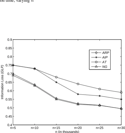
In this experiments, we set privacy levelℓ=5. With the size of the datasetnincrease, the execution time and theGLPvalues of four methods are shown in Fig. 3 and Fig. 4.
(1) Withnincrease, the execution times of the four methods are increasing, as shown in Fig.3. Among them, the execution time ofNGis always highest while the execution times ofATandAIPare less than that ofNGandARP.
(2) Withn increase, the GLP of four methods are decreasing, as shown in Fig.4. Obviously, the GLPof AT is always the maximal, while the GLPof NGandARPare always less than that ofAIPandAT.
2) The analysis of the experimental results
(1) For the experimental result (1), withnincrease, there are more records need be anonymized, so the execution times of four methods are increasing. Comparing withNG
and ARP, the anonymization of AIP is directly applied on the initial partition, so the execution time ofAIPis less than that ofARPandNG. The execution times ofARPis less than that ofNG, asNGseparately anonymizes theNSAsof each record of each block of initial partition, butARPentirety anonymizes theNSAsof the records of each sub-blocks. (2) For the experimental result (2), withnincrease, there are more records with the sameNSAsvalues in original data table, and the size of theSAvalue-set consisted of the
SAvalues of the records with the sameNSAsvalues is increasing. Thus, the probability that each recordttakesSAvalues in value-setSt(consisted of theSAvalues of the records
having the sameNSAsvalues witht) is increasing (S−Stis decreasing), so theGLPof
four methods are decreasing.
AsATdoes not take into account that put the records with sameNSAsvalues into same blocks, in the anonymized data ofAT, the probability that each recordtis assigned to the
SAin value-set (St) is small. Thus, in the samenvalues, theGLPofAT is always the
n=5 n=10 n=15 n=20 n=25 n=30 0
0.1 0.2 0.3 0.4 0.5 0.6
n (in thousands)
Time (
Second)
ARP AIP AT NG
Fig. 3.Execution time; varyingn
n=5 n=10 n=15 n=20 n=25 n=30
0.4 0.45 0.5 0.55 0.6 0.65 0.7 0.75 0.8 0.85 0.9
n (in thousands)
Information Loss (
GLP)
ARP AIP AT NG
blocks, so, in the samenvalues, theGLPofAIPis smaller than that ofAT. However, in the blocks ofAIP, there always are more thanℓrecords, and the records with different
NSAs values would be divided into the same block due to neighbor block merging (to meet the anonymizing demands ofℓ-diversity). Therefore, in the samenvalues, theGLP
value ofAIPis always more than that ofNGandARP. AsNGandARPare based on the same initial partition (generated by our method), and in the anonymized data of the two methods, the probabilities that individuals are assigned to their actualSAvalues are local maximal, theGLPvalues ofNGandARPare almost the same in statistical sense.
5.3. Varying the Size ofNSAs
1) Experimental results
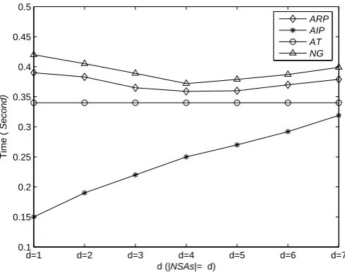
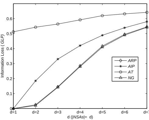
In this experiments, we set the privacy levelℓ=5 and set the size of a datasetn= 20 thousands. With the size (d) of theNSAsof the dataset increase, the execution times and theGLPvalues of four methods are shown in Fig. 5 and Fig. 6.
As stated above, there are 8 attributes in the above experiments datasetT, and the
Occuption is taken as SA, the other attributes are taken as NSAs. The correlations are computed by the mean-square contingency coefficient (as mentioned in Section IV). As-sume that theNSAssorting by the correlations (betweenNSAsandSAinT) in ascending areA1, A2, . . . , A7. We respectively project attributes,A1SA, A1A2SA, A1A2A3SA,. . ., A1A2A3A4A5A6A7SA, fromT as experimental datasetsT1, T2, . . . , T7. Thus, the size (d) of theNSAsinT1is 1 (i.e.,d= 1), the size (d) of theNSAsinT2is 2 (i.e.,d= 2), . . . , the size (d) of theNSAsinT7is 1 (i.e.,d= 7).
The anonymized datasets of the 7 datasets (T1, T2, . . . , T7) respectively are generated by the four methods, the execution time and the GLP values of the four methods are shown in Fig. 5 and Fig. 6. Theabscissa1 is the anonymized dataset ofT1,abscissa2 is the anonymized dataset ofT2, . . . ,theabscissa7 is the anonymized dataset ofT7.
(1) With the size (d) ofNSAsincrease, the execution time ofAIPincrease, and the execution time of AT is invariable. Yet, the execution times of ARP andNGdecrease at first, and then increase, as shown in Fig.5. Among them the execution time ofNGis always highest, the execution time ofAIPis always lowest, while the execution time of
ARPis more than that ofAIPandAT.
(2) With the size (d) ofNSAsincrease, theGLP of four methods are increasing, as shown in Fig.6. Among them, theGLPofATis always highest, while theGLPofNGand
ARPare less than that ofAIP. TheGLPofNGandARPare almost the same in statistical sense, and their values are always minimal.
2) The analysis of the experimental results
(1) For the experimental result (1), with the size (d) ofNSAsincrease, moreNSAsare used in recursively partition, so the initial partition ofAIP,ARPandNGconsume more times.AIPdirectly anonymize the records on the initial partition, so the execution time of
times ofARPandNGdecrease at first, and then increase. As stated above,ARPalways spends less time than that ofNG, asARPentirety anonymizes theNSAsof the records of each sub-blocks. AsATdoes not consider theNSAsof the records, the execution time of
ATis invariable.
d=1 d=2 d=3 d=4 d=5 d=6 d=7
0.1 0.15 0.2 0.25 0.3 0.35 0.4 0.45 0.5
d (|NSAs|= d)
Time (
Second)
ARP AIP AT NG
Fig. 5.Execution time; varyingd
(2) For the experimental result (2), with the size (d) ofNSAsincrease, there are less records with the sameNSAsvalues in original data table, the size of theSAvalue-set con-sisted of theSAvalues of the records with the sameNSAsvalues is decreasing. Thus, the probability that each recordttakesSAvalues in value-setSt(consisted of theSAvalues
of the records having the same NSAs values with t) is decreasing (S−St is
increas-ing), so theGLPof four methods are increasing. As stated above, Algorithm 1 ensures that the records with the sameNSA(having more interrelated withSA) values are divided into same blocks, and without loss generality, we also generate the partition of NGby Algorithm 1, so anonymization on the records of the blocks causes less correspondence loss, especially whiled = 1, the records with the sameA1 values are divided into the same blocks, theGLPvalues ofARP,AIPandNGare zero. In addition, as stated above, anonymization on refined partition causes the higher probability that records are assigned to their actualSAvalues in the anonymized tables, so theGLPofNGandARPare less then that ofAIP. AsATdoes not consider theNSAsof the records, theGLPofATalways is higher than that of the other methods.
d=1 d=2 d=3 d=4 d=5 d=6 d=7 0
0.1 0.2 0.3 0.4 0.5 0.6
d (|NSAs|= d)
Information Loss (
GLP)
ARP AIP AT NG
Fig. 6.The correspondences loss (GLP); varyingd
6.
Conclusions and Future work
An approach of anonymizing on the refining partition of initial partition (ARP) has been constructed, so that in same privacy levelARPpreserves more utility than anonymization on the initial partition (AIP). In addition,ARPhas more utility than that ofAT. A method of initial partition also has been design, although in same privacy level and initial partition
ARPandNGhave almost the same information loss in statistical sense,ARPspends less times than that of NG, andARP can be used for slicing, anatomy, randomization and generalization, etc., butNGonly is used for generalization.
For future work, we may consider to optimize the partition of the dataset with multiple sensitive attributes, and apply our approach in practical privacy preserving data publish-ing.
Acknowledgment.We would like to thank the experts of ICSAI 2014 for their insightful com-ments. This research is supported by National Science and Technology Major Project of China: Research on the Secure database management system and advanced technology. The project num-ber is 2010ZX01042-001-003-03.
References
1. Benjamin C. M., F., Ke, W., Rui, C., Philip S., Y.: Privacy-preserving data publishing: A survey of recent developments. Acm Computing Surveys 42(4), 2623–2627 (2010)
2. Chaytor, R., Ke, W.: Small domain randomization: same privacy, more utility. In: Proceedings of International Conference on Very Large DataBases. pp. 608–618. ACM, Singapore (2010) 3. Chi Wing, W., Jiuyong, L., Wai Chee, F., Ke, W.: (, k)-anonymity: an enhanced k-anonymity
4. Cramer, H.: Mathematical methods of statistics. Princeton, USA (1948)
5. D. J. Martin, D. Kifer, A.M.J.G., Halpern, J.Y.: Worst-case background knowledge for privacy-preserving data publishing. In: Proceedings of IEEE 23rd International Conference on Data Engineering. pp. 126 – 135. IEEE Computer Society, Istanbul, Turkey (2007)
6. Ghinita, G., Kalnis, P.: Fast data anonymization with low information loss. In: Proceedings of International Conference on Very Large DataBases. pp. 758–769. ACM, Austria (2007) 7. Gionis, A., Mazza, A., Tassa, T.: k-anonymization revisited. In: Proceedings of the 24th IEEE
International Conference on Data Engineering (ICDE). pp. 744–753. IEEE Computer Society, Cancun, Mexico (2008)
8. Hong, Z., Shengli, T., Kevin, L.: Privacy preserving data publication with features of indepen-dent l-diversity. Computer Journal 58(4), 549–571 (2014)
9. Hong, Z., Shengli, T., Meiyi, X.: Anonymization on refining partition: Same privacy, more utility. In: 2014 2nd International Conference on Systems and Informatics (ICSAI). pp. 998 – 1005. IEEE Computer Society, Shanghai China (2014)
10. http://archive.ics.uci.edu/ml/:
11. Junqiang, L., Ke, W.: On optimal anonymization for l+ -diversity. In: Proceedings of the IEEE 26th International Conference on Data Engineering (ICDE). pp. 213–224. IEEE Computer So-ciety, Long Beach, California, USA (2010)
12. Ke, W., Chao, H., Fu, A.W.: Randomization resilient to sensitive reconstruction. arXiv preprint arXiv:1202.3179 (2012)
13. Li, T., Li, N., JianZhang, Ian, M.: Slicing: A new approach for privacy preserving data publish-ing. IEEE Transactions on Knowledge and Data Engineering 24(3), 561–674 (2010)
14. Machanavajjhala, A., Gehrke, J., Kifer, D.: L-diversity: privacy beyond k-anonymity. In: Pro-ceedings of the 22nd International Conference on Data Engineering. pp. 24–24. IEEE Com-puter Society, Atlanta, GA, USA (2006)
15. Machanavajjhala, A., Kifer, D., Gehrke, J., Venkitasubramaniam, M.: L-diversity: privacy be-yond k-anonymity. ACM Transactions on Knowledge Discovery from Data 1(1), 1–47 (2007) 16. Qing, Z., Koudas, N., Srivastava, D., Ting, Y.: Aggregate query answering on anonymized
tables. In: Proceedings of IEEE 23rd International Conference on Data Engineering. pp. 116– 125. IEEE Computer Society, Istanbul, Turkey (2007)
17. Terrovitis, M., Mamoulis, N., Liagouris, J., Skiadopoulos, S.: Privacy preservation by disasso-ciation. Proceedings of the VLDB Endowment 5(10), 944–955 (2012)
18. Wai Chee, F., Jia, W., Ke, W., Chi Wing, W.: Small count privacy and large count utility in data publishing. Eprint Arxiv 50(8), 20–31 (2012)
19. Wai Kit, W., Mamoulis, N., David Wai Lok, C.: Non-homogeneous generalization in privacy preserving data publishing. In: Proceedings of the ACM SIGMOD International Conference on Management of Data. pp. 139–150. ACM, Indianapolis, Indiana, USA (2010)
20. Xiaokui, X., Yufei, T.: Anatomy: Simple and effective privacy preservation. In: Proceedings of International Conference on Very Large Data Bases. pp. 139–150. ACM, Seoul, Korea (2006) 21. Xiaokui, X., Yufei, T., Nick, K.: Transparent anonymization: Thwarting adversaries who know
the algorithm. Acm Transactions on Database Systems 35(2), 1–48 (2010)
22. Xin, J., Nan, Z., Gautam, D.: Algorithm-safe privacy-preserving data publishing. In: Proceed-ings of International Conference on Extending Database Technology. pp. 633–466. ACM, In-dianapolis, Indiana, USA (2010)
Shengli Tian, Ph.D. He is currently an associate Professor in School of Information Engi-neering at Xuchang University. He received B.S. degree in Computer Science Education from Xinyang Normal University in 2002, the M.Sc. degree from Henan University in 2007, and the Ph.D. degree from Huazhong University of Science and Technology in 2014. He research interests include information security technology and machine learn-ing, etc. Email: [email protected]
Genyuan Du, Ph.D. He is currently an associate Professor in the International School of Education at Xuchang University. He received B.S. degree in Computer Science and Technology from Henan Normal University in 1997, and the M.E. degree in Signal and Information Processing from Chengdu University of Technology in 2005, and the Ph.D. degree in the college of Information Engineering at Chengdu University of Technology in 2011. Research area: Parallel computing, Image retrieval, Spatial data mining, remote sensing image processing, remote sensing and computer networks. Mr. Genyuan Du is a senior member of the CCF. Email: [email protected]
Meiyi Xie is a lecturer in School of Computer Science and Technology in Huazhong University of Science and Technology. Her research interests include data security and big data processing. Email: [email protected]