Improving SVM (Support vector Machine) for classification of images based on tree and non-tree images with Neural Network technique for Tree Detection

(1)

IJSRSET162690 | Received : 01 Dec 2016 | Accepted : 08 Dec. 2016 | November-December-2016 [(2) 6: 361-365]

361

Improving SVM (Support vector Machine) for classification of

images based on tree and non-tree images with Neural Network

technique for Tree Detection

Prof. Divyanshu Rao, Deepti Thakur

Shri Ram Institute of Technology, Jabalpur, Madhya Pradesh, India

ABSTRACT

This paper compares two different techniques of tree recognition and explains the steps of extracting tree from image, palette formation and conditioning of palette for matching. The focus of the paper is in finding the suitable method for tree recognition on the basis of recognition time, recognition rate, false detection rate, conditioning time, algorithm complexity, bulk detection, database handling. The two methods compared in this paper. Although both methods are practically proven by many researchers, still a comprehensive comparison is missing, we hope the results drawn in this paper will be helpful for the peoples working in same field, the complete algorithm is developed in Matlab for classification of images.

Keywords : Tree Recognition, SVM (Support Vector Machine), Neural Network, MATLAB

I. INTRODUCTION

This presents presents a novel classification based tree detection method for autonomous navigation in forest environment. The fusion of color, and texture cues has been used to segment the image into tree trunk and background objects. The segmentation of forest images into tree trunk and background objects is a challenging task due to high variations of illumination, effect of different color shades, non-homogenous bark texture, shadows and foreshortening. To accomplish this, the attempt have been made in researching the best methodology among different combinations of color, and texture descriptors, and two classification techniques to detect nearby trees and estimate the distance between forest vehicle and the base of segmented trees using monocular vision.

A simple heuristic distance measurement method is proposed that is based on pixel height and a reference length. The performance of various color and texture operators, and accuracy of classifiers has been evaluated using cross validation techniques.

II. METHODS AND MATERIAL

2. Preprocessing for tree recognition

Tree Once the image is captured, the image is resized to 320x240 pixels in resolution. This step is done both to speed up the image processing and tree detection procedure. In experiments we have observed that images with 320x240 size still preserve good enough color and texture information. We have collected three different data bases as described in Chapter 5. Most of the images used as examples for tree detection and distance measurement in this chapter are from image database II, which has been collected in winter season for experiments.

2.1 Image Smoothing

If needed, a gaussian smoothing filter with 5x5 kernel size is applied and the number of colors in the image is reduced in order to make the system faster.

2.2 Color Transformation

(2)

3. Support Vector Machine (SVM) Classification

Support vector machines and other kernel-based methods has become a popular tool in many kinds of machine learning tasks. In audio processing, SVMs have been used, for example, in phonetic segmentation, speech recognition, and general audio classification. One advantage of SVMs is their accuracy and superior generalization properties they offer when compared to many other types of

classifiers. SVMs are based on statistical learning

theory and structural risk minimization. In the following section a brief introduction to SVM classification operation is presented when applied to binary and multiclass cases as is done in this work.

3.1 Binary classification

Let xi ∈ Rm be a feature vector or a set of input variables and let yi ∈ {+1, −1} be a corresponding class label, where m is the dimension of the feature vector. In linearly separable cases a separating hyperplane satisfies

Where the hyperplane is denoted by a vector of weights w and a bias term b. The optimal separating hyperplane, when classes have equal loss-functions, maximizes the margin between the hyperplane and the closest samples of classes. The margin is given by

The optimal separating hyperplane can now be solved by maximizing (3) subject to (1). The solution can be found using the method of Lagrange multipliers. The objective is now to minimize the Lagrangian

and requires that the partial derivatives of w and b be zero. In (4), αi are nonnegative Lagrange multipliers. Partial derivatives propagate to constraints w = ∑i αiyixi and ∑i αiyi = 0. Substituting w into (4) gives the dual form

which is not anymore an explicit function of w or b. The optimal hyperplane can be found by maximizing (5) subject to ∑i αiyi = 0 and all Lagrange multipliers are nonnegative. However, in most real world situations classes are not linearly separable and it is not possible to find a linear hyperplane that would satisfy (1) for all i = 1. . . n. In these cases a classification problem can be made linearly separable by using a nonlinear mapping into the feature space where classes are linearly separable. The condition for perfect classification can now be written as

where Φ is the mapping into the feature space. Note that the feature mapping may change the dimension of the feature vector. The problem now is how to find a suitable mapping Φ to the space where classes are linearly separable. It turns out that it is not required to know the mapping explicitly as can be seen by writing (6) in the dual form

and replacing the inner product in (7) with a suitable kernel function K(xj , xi) = (Φ(xj) · Φ(xi)). This form arises from the same procedure as was done in the linearly separable case that is, writing the Lagrangian of (6), solving partial derivatives, and substituting them back into the Lagrangian. Using a kernel trick, we can remove the explicit calculation of the mapping Φ and need to only solve the Lagrangian (5) in dual form, where the inner product (xi · xj) has been transposed with the kernel function in nonlinearly separable cases. In the solution of the Lagrangian, all data points with nonzero (and nonnegative) Lagrange multipliers are called support vectors (SV).

(3)

The slack variable is adjusted by the regularization constant C, which determines the tradeoff between complexity and the generalization properties of the classifier. This limits the Lagrange multipliers in the dual objective function (5) to the range 0 ≤ αi ≤ C. Any function that is derived from mappings to the feature space satisfies the conditions for the kernel function.

3.2. Multiclass classification

The above discussion only covers the binary classification case, which is insufficient for our situation. There are several ways to construct SVM classifiers for more than two classes. Methods can be divided into sub methods that use only one decision function, or into methods that solve many binary problems, the latter being more common. Furthermore, methods comprising multiple binary classifiers can be constructed in many ways. In this work, we use a one against one method. Each classifier performs classification between two classes and we add vote for that class. Finally, at the end, the highest voted class is considered as the winning class.

3.2 Neural Network

The term neural network was traditionally used to refer to a network or circuit of biological neurons. The modern usage of the term often refers to artificial neural networks, which are composed of artificial neurons or nodes. Thus the term has two distinct usages:

1. Biological neural networks are made up of real biological neurons that are connected or functionally related in the peripheral nervous system or the central nervous system. In the field of neuroscience, they are often identified as groups of neurons that perform a specific physiological function in laboratory analysis. 2. Artificial neural networks are composed of interconnecting artificial neurons (programming constructs that mimic the properties of biological neurons). Artificial neural networks may either be used to gain an understanding of biological neural networks, or for solving artificial intelligence problems without necessarily creating a model of a real biological system. The real, biological nervous system is highly complex: artificial neural network algorithms attempt to abstract this complexity and

focus on what may hypothetically matter most from an information processing point of view. Good performance (e.g. as measured by good predictive ability, low generalization error), or performance mimicking animal or human error patterns, can then be used as one source of evidence towards supporting the hypothesis that the abstraction really captured something important from the point of view of information processing in the brain. Another incentive for these abstractions is to reduce the amount of computation required to simulate artificial neural networks, so as to allow one to experiment with larger networks and train them on larger data sets.

An artificial neural network (ANN), usually called neural network (NN), is a mathematical model or computational model that is inspired by the structure and/or functional aspects of biological neural networks. A neural network consists of an interconnected group of artificial neurons, and it processes information using a connectionist approach to computation. In most cases an ANN is an adaptive system that changes its structure based on external or internal information that flows through the network during the learning phase. Modern neural networks are non-linear statistical data modeling tools. They are usually used to model complex relationships between inputs and outputs or to find patterns in data.

An tree-recognition algorithm first a discrete cosine transform is used in order to extract the spatial frequency range that contains the main abstract of tree image. The result is a set of complex numbers that carry local amplitude and phase information for the tree image which is used as training input for neural network.

(4)

of the competitive neural networks. Following figure shows the structure of neural network:

Figure 1. Structure of neural network

4. Proposed Algorithm

Here we detail a new algorithm for classification of PD (Partial Discharge).

Step 1: resize the image into 128X128 pixels Step 2: Take the RGB planes of input image. Step 3: Convert each plane to 8X8 pixel blocks. Step 4: Take 2-D DCT of each block.

Step 5: Take only first three components from each block.

Step 6: Arrange first three components from each block into a single row matrix as training vector.

Step 7: Calculate the same matrix for all images. Step 8: Assign label to each matrix according to their

class.

Step 9: Train SVM using one against one method & create n*(n – 1)/2 classifiers, where n is total number of classes.

Step 10: To classify a new PD pattern first repeat the steps 1 to 6 to create the vector.

Step 11: Collect the votes using above trained classifiers.

Step 12: Take the decision in favor of class which gets the maximum votes.

III. RESULTS AND DISCUSSION

The simulation results of the implemented algorithm, all the simulation is performed with intel P4 1.4 GHz processors with 1 GB of RAM, the OS is windows and simulation software is MATLAB 7.5(R2007b).

The figure 2 shows the comparative analysis of training time taken by two methods for three different tree images and each having samples from 3 to 10. The graph shows that SVM takes slightly greater time then NN because of long time taken for calculation of correlation.

Figure 2. Samples Vs. Training Time

The figure 2 shows the comparative analysis of training time taken by two methods for 3 to 10 different tree images and each having three samples. The graph shows that time taken by SVM increases in linear way as the number of tree images increases then NN which drops the slope because NN trains in different way.

Figure 3 number of tree vs. training time

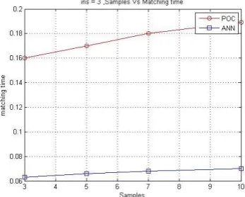
The figure 3 shows the comparative analysis of matching time taken by two methods for three different tree images and each having samples from 3 to 10. The graph shows that SVM is 3 times slower then NN. NN is fast because if forms a combinational arrangement after training.

(5)

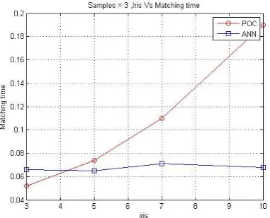
The figure 4 shows the comparative analysis of matching time taken by two methods for 3 to 10 different tree images and each having three samples. The graph shows that time taken by SVM increases exponentially as the number of tree images increases then NN which takes constant time.

Figure 5. number of tree vs. matching time

IV. CONCLUSION

Using neural networks for a personal tree recognition system is presented in this paper. A fast tree localization method using Hough transform is explained. Using this method, tree segmentation is performed in short time. Average time for tree segmentation is obtained to be 14 sec for high resolution image (768X576). Accuracy rate of tree segmentation is about 90% is achieved. The located tree after pre-processing is represented by a feature vector. Using this vector as input signal the neural network is used to recognize the tree patterns. The recognition accuracy for trained patterns is about 90%, and for the SVM it increases to 95%.

V. REFERENCES

[1] R. Plemmonsa, M. Horvatha, E. Leonhardta, P. Paucaa, S. Prasadb, "Computational Imaging Systems for Tree Recognition" Rrocessing of Spie 2014

[2] C. L. Tisse, L. Martin, L. Torres, M. Robert, "Person identification technique using human tree recognition" ST Journal of System Research Current Issue 2015.

[3] L. Ma, U. Wang, T. Tan, "Tree Recognition Based on Multichannel Gabor Filtering" The 5th Asian Conference on Computer Vision, 23-- 25 January 2013, Melbourne, Australia.

[4] R. Narayanswamy, P. E. X. Silveir, "Extended Depth-of-Field Tree Recognition System for a Workstation Environment" Proceedings of the Spied Biometric Technology for Human Identification II,Vol. 5779, pp. 41-50, Orlando, FL, 2015.

[5] Z. Wei, T. Tan and Z. Sun, "Synthesis of Large Realistic Tree Databases Using Patch-based Sampling" IEEE 2014.

[6] A. Czajka, A. Pacut, "Replay Attack Prevention for Tree Biometrics" ICCST 2015, IEEE. [7] R. Wildes, "Tree Recognition: An Emerging

Biometric Technology," Proc. IEEE, vol. 85, no. 9, pp. 1348-1363, Sept. 2014.

[8] B.V.K. Vijaya Kumar, C. Xie, and J. Thornton, "Tree Verification Using Correlation Filters," Proc. Fourth Int’l Conf. Audio- and Video-Based Biometric Person Authentication, pp. 697-705, 2013.

[9] Z. Sun, T. Tan, and X. Qiu, "Graph Matching Tree Image Blocks with Local Binary Pattern," Advances in Biometrics, vol. 3832, pp. 366-372, Jan. 2014.

[10] C.D. Kuglin and D.C. Hines, "The Phase Correlation Image Alignment Method," Proc. Int’l Conf. Cybernetics and Soc. ’75, pp. 163-165, 1975.

[11] K. Takita, T. Aoki, Y. Sasaki, T. Higuchi, and K. Kobayashi, "High-Accuracy Subpixel Image Registration Based on Phase- Only Correlation," IEICE Trans. Fundamentals, vol. E86-A, no. 8, pp. 1925-1934, Aug. 2013.

[12] K. Takita, M.A. Muquit, T. Aoki, and T. Higuchi, "A Sub-Pixel Correspondence Search Technique for Computer Vision Applications," IEICE Trans. Fundamentals, vol. 87-A, no. 8, pp. 1913-1923, Aug. 2014.

[13] K. Ito, H. Nakajima, K. Kobayashi, T. Aoki, and T. Higuchi, "A Fingerprint Matching Algorithm Using Phase-Only Correlation," IEICE Trans. Fundamentals, vol. 87-A, no. 3, pp. 682-691, Mar. 2014.